Under the background that Covid-19 is spreading across the world, the lifestyle of people has to confront a series of changes and challenges. This also presents new problems and requirements to automation facilities. For example, nowadays masks have almost become necessities for people in public places. However, most access control systems (ACS) cannot recognize people wearing masks and authenticate their identities to deal with increasingly serious epidemic pressure. Consequently, many public entries have turned to an attendant mode that brings low efficiency, infection potential, and high possibility of negligence. In this paper, a new security classification framework based on face recognition is proposed. This framework uses mask detection algorithm and face authentication algorithm with anti-spoofing function. In order to evaluate the performance of the framework, this paper employs the Chinese Academy of Science Institute of Automation-Face Anti-spoofing Datasets (CASIA-FASD) and Reply-Attack datasets as benchmarks. Performance evaluation indicates that the Half Total Error Rate (HTER) is 9.7%, the Equal Error Rate (EER) is 5.5%. The average process time of a single frame is 0.12 seconds. The results demonstrate that this framework has a high anti-spoofing capability and can be employed on the embedded system to complete the mask detection and face authentication task in real-time.
Citation: Dongzhihan Wang, Guijin Ma, Xiaorui Liu. An intelligent recognition framework of access control system with anti-spoofing function[J]. AIMS Mathematics, 2022, 7(6): 10495-10512. doi: 10.3934/math.2022585
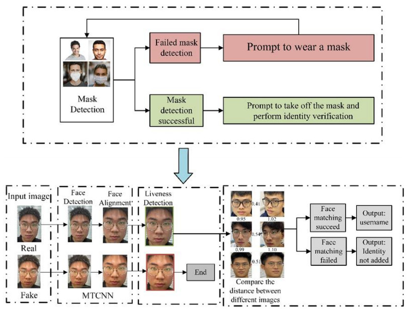
Under the background that Covid-19 is spreading across the world, the lifestyle of people has to confront a series of changes and challenges. This also presents new problems and requirements to automation facilities. For example, nowadays masks have almost become necessities for people in public places. However, most access control systems (ACS) cannot recognize people wearing masks and authenticate their identities to deal with increasingly serious epidemic pressure. Consequently, many public entries have turned to an attendant mode that brings low efficiency, infection potential, and high possibility of negligence. In this paper, a new security classification framework based on face recognition is proposed. This framework uses mask detection algorithm and face authentication algorithm with anti-spoofing function. In order to evaluate the performance of the framework, this paper employs the Chinese Academy of Science Institute of Automation-Face Anti-spoofing Datasets (CASIA-FASD) and Reply-Attack datasets as benchmarks. Performance evaluation indicates that the Half Total Error Rate (HTER) is 9.7%, the Equal Error Rate (EER) is 5.5%. The average process time of a single frame is 0.12 seconds. The results demonstrate that this framework has a high anti-spoofing capability and can be employed on the embedded system to complete the mask detection and face authentication task in real-time.

| [1] |
B. Qin, D. Li, Identifying facemask-wearing condition using image super-resolution with classification network to prevent COVID-19, Sensors, 10 (2020), 5236. https://doi.org/10.3390/s20185236 doi: 10.3390/s20185236

|
| [2] |
M. S. Ejaz, M. R. Islam, M. Sifatullah, A. Sarker, Implementation of principal component analysis on masked and non-masked face recognition, 2019 1st Int. Conf. Adv. Sci., Eng. Rob. Technol. (ICASERT), 2019, 1–5. https://doi.org/10.1109/ICASERT.2019.8934543 doi: 10.1109/ICASERT.2019.8934543
|
| [3] | M. Jiang, X. Fan, H. Yan, Retinamask: A face mask detector, arXiv, unpublished work. |
| [4] |
J. Hosang, R. Benenson, B. Schiele, Learning non-maximum suppression, 2017 IEEE Conf. Comput. Vision Pattern Recognit. (CVPR), 2017, 4507–4515. https://doi.org/10.1109/CVPR.2017.685 doi: 10.1109/CVPR.2017.685
|
| [5] | S. Woo, J. Park, J. Lee, I. Kweon, Cbam: Convolutional block attention module, Proc. Eur. Conf. Comput. Vision (ECCV), 2018, 3–19. |
| [6] | Y. Taigman, M. Yang, M. A. Ranzato, L. Wolf, Deepface: Closing the gap to human-level performance in face verification, Proc. IEEE Conf. Comput. Vision Pattern Recognit. (CVPR), 2014, 1701–1708. |
| [7] | Y. Sun, X. Wang, X. Tang, Deep learning face representation from predicting 10,000 classes, Proc. IEEE Conf. Comput. Vision Pattern Recognit. (CVPR), 2014, 1891–1898. |
| [8] |
D. Nguyen, K. Nguyen, S. Sridharan, D. Dean, C. Fookes, Deep spatio-temporal feature fusion with compact bilinear pooling for multimodal emotion recognition, Comput. Vis. Image Und., 174 (2018), 33–42. https://doi.org/10.1016/j.cviu.2018.06.005 doi: 10.1016/j.cviu.2018.06.005
|
| [9] | J. Deng, J. Guo, N. Xue, S. Zafeiriou, Arcface: Additive angular margin loss for deep face recognition, Proc. IEEE/CVF Conf. Comput. Vision Pattern Recognit. (CVPR), 2019, 4690–4699. |
| [10] | H. Liu, X. Zhu, Z. Lei, S. Z. Li, Adaptiveface: Adaptive margin and sampling for face recognition, Proc. IEEE/CVF Conf. Comput. Vision Pattern Recognit. (CVPR), 2019, 11947–11956. |
| [11] |
Y. Jiang, W. Li, M. S. Hossain, M. Chen, A. Alelaiwi, M. Al-Hammadi, A snapshot research and implementation of multimodal information fusion for data-driven emotion recognition, Inform. Fusion, 53 (2019), 145–156. https://doi.org/10.1016/j.inffus.2019.06.019 doi: 10.1016/j.inffus.2019.06.019
|
| [12] | Y. Huang, Y. Wang, Y. Tai, X. Liu, P. Shen, S. Li, et al., Curricularface: Adaptive curriculum learning loss for deep face recognition, Proc. IEEE/CVF Conf. Comput. Vision Pattern Recognit. (CVPR), 2020, 5901–5910. |
| [13] |
Z. Boulkenafet, J. Komulainen, A. Hadid, Face anti-spoofing based on color texture analysis, 2015 IEEE Int. Conf. Image Proc. (ICIP), 2015, 2636–2640. https://doi.org/10.1109/ICIP.2015.7351280 doi: 10.1109/ICIP.2015.7351280
|
| [14] |
Z. Boulkenafet, J. Komulainen, A. Hadid, Face spoofing detection using colour texture analysis, IEEE T. Inf. Forensics Secur., 11 (2016), 1818–1830. https://doi.org/10.1109/TIFS.2016.2555286 doi: 10.1109/TIFS.2016.2555286
|
| [15] |
X. Li, J. Komulainen, G. Zhao, P. C. Yuen, M. Pietikäinen, Generalized face anti-spoofing by detecting pulse from face videos, 2016 23rd Int. Conf. Pattern Recognit. (ICPR), 2016, 4244–4249. https://doi.org/10.1109/ICPR.2016.7900300 doi: 10.1109/ICPR.2016.7900300
|
| [16] | I. Chingovska, N. Erdogmus, A. Anjos, S. Marcel, Face recognition systems under spoofing attacks, In: T. Bourlai, Face recognition across the imaging spectrum, Springer, 2016, 165–194. https://doi.org/10.1007/978-3-319-28501-6_8 |
| [17] | S. Q. Liu, X. Lan, P. C. Yuen, Remote photoplethysmography correspondence feature for 3D mask face presentation attack detection, Proc. Eur. Conf. Comput. Vision (ECCV), 2018,558–573. |
| [18] |
I. Manjani, S. Tariyal, M. Vatsa, R. Singh, A. Majumdar, Detecting silicone mask-based presentation attack via deep dictionary learning, IEEE T. Inf. Forensics Secur., 2017, 1713–1723. https://doi.org/10.1109/TIFS.2017.2676720 doi: 10.1109/TIFS.2017.2676720
|
| [19] |
R. Shao, X. Lan, P. C. Yuen, Joint discriminative learning of deep dynamic textures for 3d mask face anti-spoofing, IEEE T. Inf. Forensics Secur., 14 (2018), 923–938. https://doi.org/10.1109/TIFS.2018.2868230 doi: 10.1109/TIFS.2018.2868230
|
| [20] |
J. Määttä, A. Hadid, M. Pietikäinen, Face spoofing detection from single images using micro-texture analysis, 2011 Int. Joint Conf. Biometrics (IJCB), 2011, 1–7. https://doi.org/10.1109/IJCB.2011.6117510 doi: 10.1109/IJCB.2011.6117510
|
| [21] |
J. Määttä, A. Hadid, M. Pietikäinen, Face spoofing detection from single images using texture and local shape analysis, IET Biom., 1 (2012), 3–10. https://doi.org/10.1049/iet-bmt.2011.0009 doi: 10.1049/iet-bmt.2011.0009
|
| [22] |
Y. Atoum, Y. Liu, A. Jourabloo, X. Liu, Face anti-spoofing using patch and depth-based CNNs, 2017 IEEE International Joint Conference on Biom. (IJCB), 2017,319–328. https://doi.org/10.1109/BTAS.2017.8272713 doi: 10.1109/BTAS.2017.8272713
|
| [23] | Y. Liu, A. Jourabloo, X. Liu, Learning deep models for face anti-spoofing: Binary or auxiliary supervision, Proc. IEEE Conf. Comput. Vision Pattern Recognit. (CVPR), 2018,389–398. |
| [24] |
G. Pan, L. Sun, Z. Wu, S. Lao, Eyeblink-based anti-spoofing in face recognition from a generic web camera, 2007 IEEE 11th Int. Conf. Comput. Vision, 2007, 1–8. https://doi.org/10.1109/ICCV.2007.4409068 doi: 10.1109/ICCV.2007.4409068
|
| [25] | A. Zadeh, P. P. Liang, N. Mazumder, S. Poria, E. Cambria, L. P. Morency, Memory fusion network for multi-view sequential learning, Thirty-Second AAAI Conf. Artif. Intell., 32 (2018), 5642–5649. |
| [26] |
T. Baltruaitis, C. Ahuja, L. P. Morency, Multimodal machine learning: A survey and taxonomy, IEEE T. Pattern Anal. Mach. Intell., 41 (2019), 154–163. https://doi.org/10.1109/TPAMI.2018.2798607 doi: 10.1109/TPAMI.2018.2798607
|
| [27] | T. Li, Q. Yang, S. Rong, L. Chen, B. He, Distorted underwater image reconstruction for an autonomous underwater vehicle based on a self-attention generative adversarial network, Appl. Opt., 59 (2020), 10049–10060. |
| [28] |
T. Li, S. Rong, X. Cao, Y. Liu, L. Chen, B. He, Underwater image enhancement framework and its application on an autonomous underwater vehicle platform, Opt. Eng., 59 (2020), 083102. https://doi.org/10.1117/1.OE.59.8.083102 doi: 10.1117/1.OE.59.8.083102
|
| [29] |
K. Zhang, Z. Zhang, Z. Li, Y. Qiao, Joint face detection and alignment using multitask cascaded convolutional networks, IEEE Signal Proc. Let., 23 (2016), 1499–1503. https://doi.org/10.1109/LSP.2016.2603342 doi: 10.1109/LSP.2016.2603342
|
| [30] | J. Fu, J. Liu, H. Tian, Y. Li, Y. Bao, Z. Fang, et al., Dual attention network for scene segmentation, Proc. IEEE/CVF Conf. Comput. Vision Pattern Recognit. (CVPR), 2019, 3146–3154. |
| [31] |
W. Sanghyun, H. Soonmin, I. S. Kweon, Stairnet: Top-down semantic aggregation for accurate one-shot detection, 2018 IEEE Winter Conf. Appl. Comput. Vision (WACV), 2018, 1093–1102. https://doi.org/10.1109/WACV.2018.00125 doi: 10.1109/WACV.2018.00125
|
| [32] | T. Ojala, M. Pietikäinen, T. Mäenpää, Gray scale and rotation invariant texture classification with local binary patterns, In: Computer Vision-ECCV 2000, Lecture Notes in Computer Science, Springer, 1842 (2000), 404–420. https://doi.org/10.1007/3-540-45054-8_27 |
| [33] |
T. Ojala, M. Pietikainen, T. Maenpaa, Multiresolution gray-scale and rotation invariant texture classification with local binary patterns, IEEE T. Pattern Anal. Mach. Intell., 24 (2002), 971–987. https://doi.org/10.1109/TPAMI.2002.1017623 doi: 10.1109/TPAMI.2002.1017623
|
| [34] |
W. S. Noble, What is a support vector machine? Nat. Biotechnol., 24 (2006), 1565–1567. https://doi.org/10.1038/nbt1206-1565 doi: 10.1038/nbt1206-1565
|
| [35] | F. N. Iandola, S. Han, M. W. Moskewicz, K. Ashraf, W. J. Dally, K. Keutzer, SqueezeNet: AlexNet-level accuracy with 50x fewer parameters and < 0.5 MB model size, arXiv, unpublished work. |
| [36] | F. Chollet, Xception: Deep learning with depthwise separable convolutions, Proc. IEEE Conf. Comput. Vision Pattern Recognit. (CVPR), 2017, 1251–1258. |
| [37] | M. Sandler, A. Howard, M. Zhu, A. Zhmoginov, L. C. Chen, Mobilenetv2: Inverted residuals and linear bottlenecks, Proc. IEEE Conf. Comput. Vision Pattern Recognit. (CVPR), 2018, 4510–4520. |
| [38] | A. Howard, M. Sandler, G. Chu, L. C. Chen, B. Chen, M. Tan, et al., Searching for mobilenetv3, Proc. IEEE/CVF Int. Conf. Comput. Vision (ICCV), 2019, 1314–1324. |
| [39] | N. Ma, X. Zhang, H. Zheng, J. Sun, Shufflenet v2: Practical guidelines for efficient CNN architecture design, Proc. Eur. Conf. Comput. Vision (ECCV), 2018,116–131. |
| [40] |
Z. Zhang, J. Yan, S. Liu, Z. Lei, D. Yi, S. Z. Li, A face antispoofing database with diverse attacks, 2012 5th IAPR Int. Conf. Biom. (ICB), 2012, 26–31. https://doi.org/10.1109/ICB.2012.6199754 doi: 10.1109/ICB.2012.6199754
|
| [41] |
A. Costa-Pazo, S. Bhattacharjee, E. Vazquez-Fernandez, Sebastien Marcel, The replay-mobile face presentation-attack database, 2016 Int. Conf. Biom. Spec. Interest Group (BIOSIG), 2016, 1–7. https://doi.org/10.1109/BIOSIG.2016.7736936 doi: 10.1109/BIOSIG.2016.7736936
|


Figures(9) / Tables(2)

Dongzhihan Wang, Guijin Ma, Xiaorui Liu. An intelligent recognition framework of access control system with anti-spoofing function[J]. AIMS Mathematics, 2022, 7(6): 10495-10512. doi: 10.3934/math.2022585


 DownLoad: