


Figure1.
A cell environment.
In this note, our purpose is to introduce the concept of -polynomial convex stochastic processes and study some of their algebraic properties. We establish new refinements for integral version of Hölder and power mean inequality. Also, we are concerned to extend several Hermite-Hadamard type inequalities for -polynomial convex stochastic processes by using Hölder, Hölder-İşcan, power mean and improved power mean integral inequalities. Moreover, we give comparison of obtained results.
Citation: Haoliang Fu, Muhammad Shoaib Saleem, Waqas Nazeer, Mamoona Ghafoor, Peigen Li. On Hermite-Hadamard type inequalities for -polynomial convex stochastic processes[J]. AIMS Mathematics, 2021, 6(6): 6322-6339. doi: 10.3934/math.2021371
| [1] | Mengting Sui, Yanfei Du . Bifurcations, stability switches and chaos in a diffusive predator-prey model with fear response delay. Electronic Research Archive, 2023, 31(9): 5124-5150. doi: 10.3934/era.2023262 |
| [2] | Yujia Xiang, Yuqi Jiao, Xin Wang, Ruizhi Yang . Dynamics of a delayed diffusive predator-prey model with Allee effect and nonlocal competition in prey and hunting cooperation in predator. Electronic Research Archive, 2023, 31(4): 2120-2138. doi: 10.3934/era.2023109 |
| [3] | Jiani Jin, Haokun Qi, Bing Liu . Hopf bifurcation induced by fear: A Leslie-Gower reaction-diffusion predator-prey model. Electronic Research Archive, 2024, 32(12): 6503-6534. doi: 10.3934/era.2024304 |
| [4] | Fengrong Zhang, Ruining Chen . Spatiotemporal patterns of a delayed diffusive prey-predator model with prey-taxis. Electronic Research Archive, 2024, 32(7): 4723-4740. doi: 10.3934/era.2024215 |
| [5] | Yichao Shao, Hengguo Yu, Chenglei Jin, Jingzhe Fang, Min Zhao . Dynamics analysis of a predator-prey model with Allee effect and harvesting effort. Electronic Research Archive, 2024, 32(10): 5682-5716. doi: 10.3934/era.2024263 |
| [6] | Xiaowen Zhang, Wufei Huang, Jiaxin Ma, Ruizhi Yang . Hopf bifurcation analysis in a delayed diffusive predator-prey system with nonlocal competition and schooling behavior. Electronic Research Archive, 2022, 30(7): 2510-2523. doi: 10.3934/era.2022128 |
| [7] | Miao Peng, Rui Lin, Zhengdi Zhang, Lei Huang . The dynamics of a delayed predator-prey model with square root functional response and stage structure. Electronic Research Archive, 2024, 32(5): 3275-3298. doi: 10.3934/era.2024150 |
| [8] | Yuan Tian, Yang Liu, Kaibiao Sun . Complex dynamics of a predator-prey fishery model: The impact of the Allee effect and bilateral intervention. Electronic Research Archive, 2024, 32(11): 6379-6404. doi: 10.3934/era.2024297 |
| [9] | Kimun Ryu, Wonlyul Ko . Global existence of classical solutions and steady-state bifurcation in a prey-taxis predator-prey system with hunting cooperation and a logistic source for predators. Electronic Research Archive, 2025, 33(6): 3811-3833. doi: 10.3934/era.2025169 |
| [10] | Yuan Tian, Hua Guo, Wenyu Shen, Xinrui Yan, Jie Zheng, Kaibiao Sun . Dynamic analysis and validation of a prey-predator model based on fish harvesting and discontinuous prey refuge effect in uncertain environments. Electronic Research Archive, 2025, 33(2): 973-994. doi: 10.3934/era.2025044 |
In this note, our purpose is to introduce the concept of -polynomial convex stochastic processes and study some of their algebraic properties. We establish new refinements for integral version of Hölder and power mean inequality. Also, we are concerned to extend several Hermite-Hadamard type inequalities for -polynomial convex stochastic processes by using Hölder, Hölder-İşcan, power mean and improved power mean integral inequalities. Moreover, we give comparison of obtained results.
Each semester, I am systematically asked this question in my graduate and undergraduate courses. Since the major improvements in industrial biotech have came from cell engineering work, why should we spend time and effort developing complex mathematical models? The answer is obviously not straightforward or unique, and may differ depending on your respective research or industrial fields of interest. In fact, there are various examples to illustrate when the modeling of cell behavior is thought to provide a useful tool to address complex multifactorial problems. For instance, the Chinese Hamster Ovary (CHO) production cell platform is a very interesting case of study. This cell platform is now a key player on the industrial scene for the production of most biotherapeutics such as monoclonal antibodies (mAb) and other proteins [1,2]. Like microbial platforms, the most significant improvements in animal cell platforms’ productivity are generally still obtained from genetic engineering work. One or a set of genes that are directly involved in the biochemical reactions sequence leading to the compound of interest are selected, usually intuitively, and their expression levels are altered aiming at their overexpression or silencing [2]. However, the results are often the opposite of what was expected, and it is common to perform several steps of successive screenings for cell engineering targets as well as for parental and recombinant cell lines. In fact, intuition can be poor counsel for this type of work since the cellular metabolism is highly interlinked and regulated, making the result of a genetic or environmental intervention, from the modification of medium composition or of culture conditions, usually unpredictable. In order to be fully expressed, the improved capacity of recombinant cell lines then requires the design of specific culture protocols, implying the optimization of culture medium composition and management, with the addition of specific compounds during a culture (e. g. under fed-batch or perfusion culture modes). Moreover, successful cell engineering work, combined with the engineering of culture media and of fed-batch (or perfusion) culture strategies, has been shown to lead to increased accumulation levels in mAbs from few mg/L (~1980) to over ~10 g/L the last few decades [1,2].
Overall, the development of a highly productive bioprocess will thus rely on the cumulative success of a series of crucial steps, from the identification of a parental cell line of high productive potential and the identification of efficient target(s) of cell engineering, to the design of optimal culture media and culture management protocols enabling the maximization and maintenance of both cell productivity and viability all along a culture cascade. Furthermore, because each step has its specific set of selection criteria, the whole process is largely based on a multifactorial analysis of experimental data, which has encouraged the industry to develop high-throughput techniques to conduct massive assays (i.e., on a large scale in terms of the amount of treatments) varying experimental parameters at many levels [2]. However, although this approach makes it possible to scan an impressive set of conditions, high titer product accumulation does not guarantee the further scale-up of the process or the product quality (i.e., protein activity) [3]. Therefore, another question that arises is: “How can a complex mathematical model be of some help since high-throughput robotized screening platforms offer a massive assay capacity at a low cost per assay, allowing to screen for optimal culture media, high productive cell lines and target(s) for cell engineering works?” In this context of a multifactorial problem, attempts are now being made to develop predictive models capable of guiding interpretation of the resulting big datasets. Such models are thus expected to lead to major breakthroughs not only in the field of industrial biotechnology, but also in medical science for the study of metabolic diseases where huge multifactorial databases are available.
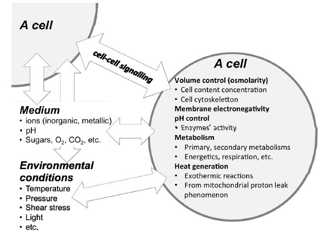
A cell evolves and interacts within an environment that stimulates or inhibits its behavior via various compounds and physico-chemical conditions (Figure 1), which all usually vary with time. In many biosystems, the use of the so-called “basic” cell culture dataset, which normally includes biomass cell concentration or optical density, and the concentration of the limiting substrate and the product suffice to describe cell growth behavior, as well as the substrate consumption and product production rates. However, access is now available to various and complementary “omics” data enabling the characterization of almost the entire cell content, biochemical reactions stoichiometry and dynamics. The temptation can thus be great to “jump on” these big datasets, but is it always necessary? A decision map (Figure 2) can be drawn to help select a modeling approach depending on your specific objective function. The graduated levels, inspired from Bloom’s learning taxonomy, show that knowledge acquisition and mathematical development can be significant, but the model complexity you will need should always depend on your specific objective function.
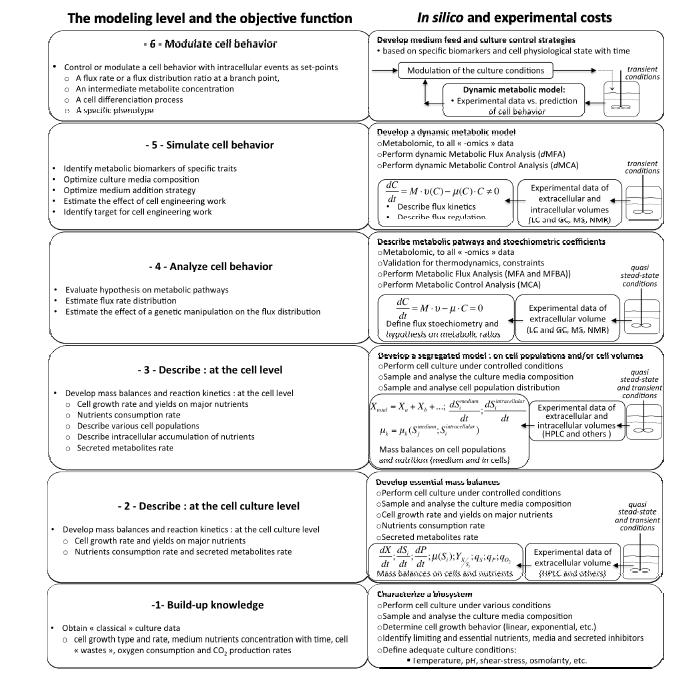
If you are simply aiming at characterizing the effect of an environment on a cell’s macroscopic behavior, you may want to start at modeling level 1, limiting your observations to traits such as cell viability, growth type and which compounds are consumed and released by the cells. Otherwise, if your goal is to characterize the interaction of cells with their environment, then you should be at level 2 and should sample and/or monitor the biosystem and acquire the experimental data necessary to compute parameters such as cell growth (or division) rate, cell yields on the major nutrients, nutrients consumption, and metabolites secretion rates (often called as wastes). There is abundant literature available for those interested in this approach and I suggest reading the early chapters of classic handbooks such as Pirt (1968) [4] and Bailey and Ollis (1986) [5]. With these data, you can develop a mathematical system made of mass balances describing the time variations of the various culture parameters for which you have experimental data. These mass balances are essentially differential equations accounting for the consumption of nutrients, the production of the compound of interest and cell growth. Since an important issue at that level is to describe reaction kinetics, the Monod (1959) [6] equation is still pertinent and useful, along with others that have since been developed [5].
At level 2 you basically obtain a simulator of macroscopic cell behavior, which requires you to know only about initial culture conditions at time “0.” The numerical integration of the system of differential equations using commercial software will do the rest, drawing a projection in time of the state of a culture. However, although level 2 is highly sufficient for many biosystems, in the case of cells accumulating compounds (e. g. plant cells [7,8]), or those composed of a set of sub-populations that need to be described, you may need to move on to level 3. The model is more complex at that level, but that is the cost of being able to describe complex cell populations.
If you systematically experience discrepancies between model simulations and your datasets, you may need to move further in describing a cell behavior by looking closely at the reaction level inside the cells. You are then at level 4 and focusing on cell metabolic organization. It is then crucial that the experimental design limits physiological stresses from the cell environment (Figure 1), or includes their description in the model. Knowing the stoichiometry of the enzymatic reactions you are describing, you can build up a set of mass balance equations, one per enzymatic reaction, limiting your study to steady state or quasi steady state biosystems. This approach allows for the performance of the Metabolic Flux Analysis (MFA) [9] of a biosystem, linking compounds in the cell environment to their intracellular processing through the metabolic network of enzymatic reactions. Adding adequate hypotheses or “constraints, ” you can draw the space of solutions for your biosystem and thus evaluate the “potential” of the cells under study using the Metabolic Flux Balance Analysis (MFBA) [10].
When reversible biochemical reactions need to be analyzed, various labeled substrates (e. g., 13C, 15N, 31O, etc. ) can be fed to the cells and the effective flux determined [9]. If you can perform specific cell engineering work modifying an enzyme activity level, you can then perform what is called a Metabolic Control Analysis (MCA) [11], and thus evaluate the metabolic flexibility or rigidity of the cells under study. At that level, you can estimate the flux distribution within a defined metabolic network. Thus, knowing the stoichiometry of the metabolic reactions, you know where carbon flows and at what rates. This is very useful since it can tell you about potential bottlenecks limiting or diverging the carbon flow from the biosynthetic pathways leading to your product of interest or towards any of your objective functions. Combined with MCA, you can then locate potential targets of cell engineering works enabling the carbon to be redirected towards your objective function (e. g., cell growth rate, production or other). However, if you are looking for a predictive capacity of cell behavior, MFBA appears to offer some potential [12], although you may need to move on to the next modeling level.
By predictive capacity you may understand “in time”, such as in transient processes or where perturbations occur, both cases that are normally encountered in many biosystems. You are then at level 5 where the complexity of this approach may become significant but the outcomes are worth it in many cases. The complexity of the approach involves not only mathematical work, but also, and primarily, obtaining the required experimental data. You need to quantify the cell intracellular content in metabolites and intermediate metabolites, data obtained using cell extraction protocols that must be highly efficient at quenching the cell metabolism in order to stop enzymatic reactions. The samples are then analyzed using sophisticated and expensive equipment with various detectors such as mass spectrometry [13,14] and nuclear magnetic resonance (NMR) [14,15]. With this approach, because you have experimental datasets as well as culture time, you can address the description of transient behaviors of metabolic events, although there is a high labor cost involved in describing the biochemical reaction kinetics, implying a set of kinetic parameters to be determined for each enzymatic reaction. In many cases, such parameters cannot be found in the literature or in databanks (e. g., BRENDA, brenda-enzymes. info [16] and references therein). And if you do find any, they may have been determined in vitro, meaning they may not correspond to the intracellular conditions of your biosystem.
The parameters that are not described in the literature and databanks have to be determined from estimations, while minimizing model simulation error compared to experimental data. Although the process may be quite laborious when the parameter number to be estimated is high, parameter values can still be identified following standard statistical analysis of the confidence intervals. Considering that such a model consists in a simplification of the biosystem’s metabolism, it is understood that the estimated kinetic parameter values can hardly be those of the enzymes in action; the more detailed a model described, the closer the parameter values to the real conditions.
In order to avoid or limit this problem, hybrid approaches have been proposed accounting for a limited set of transient reactions while keeping others at steady state [17,18]. However, these approaches show limited predictive capacity, requiring periodic re-scaling steps on freshly obtained experimental data. To be qualified as predictive, a model should be able to simulate cell behavior in time from defining initial conditions, including that of the cells. Such an in silico platform can be invaluable to perform complex tasks such as evaluating various medium compositions and medium feeding strategies. A dynamic MFC (dMFC) study can then be conducted to assess “optimal” culture strategies. For instance, the objective function can then consist in seeking to maximize carbon flow along pathways leading to a product synthesis, or for any other metabolic event. This process of simulating how each flux rate or their ratios evolve with time can also lead to the identification of specific biomarkers of a cell’s physiological state, which can then be translated into a defined combination of culture parameters that can be monitored to probe specific biosystem’s metabolic states (e. g., growth and/or production). Even from a limited set of experimental data, metabolic changes occurring with time and culture perturbations can thus be studied [19]. Accordingly, these studies can be extremely useful for improving our understanding of the cell’s intracellular dynamics against changes and perturbations in its environment [20,21].
However, the key to obtaining a predictive model may lie in the description of the various metabolic pathway regulation phenomena, which enable cell survival within a changing environment. At such a high level of modeling, dynamic MCA (dMCA) analysis can start to be performed, testing hypothesis of targets for cell engineering work. Some attempts to use such data-driven models have also been conducted to assist in defining real-time fed-batch culture strategies to control CHO [17] and plant cells’ metabolic state [22,23], to study the effect of a genetic modification on potato cell behavior [24], and to study the role of energetic robustness in mice model of Parkinson’s disease [25]. However, these studies were limited within known experimental spaces. As expected, the closer a model describes a cell’s machinery, the better its predictive capacity, and at that complexity level the outputs (i.e., simulations) of a model should still be taken as hypothetic predictions.
If your objective function is to be able to modulate cell metabolism making “live” real-time decisions on the management of a cell environment, you then need to climb to level 6. Although at a lower level (i.e., from level 4), you can increase the model’s predictive capacity by including some knowledge on proteomics, interactomics, expressomics and genomics, at level 6 this step is mandatory. It may also be required to account for physiological aspects such as those described in Figure 1. The aim here is to provide a model predictive capacity that can go beyond a known experimental space. Such a modeling level is thus expected to allow for the identification of optimal cell metabolism and cell culture management, including exploring hypotheses of therapies and biomedical approaches such as regenerative medicine.
How much should modeling approaches differ among biosystems? This is an important question that arises when initiating modeling work on a cell type with which we are unfamiliar. The normal reflex is to consider that they are all specific enough to require a distinct modeling approach. Cell genetics obviously differs among species, as do the resulting metabolomics, with different intermediate metabolites and enzymes concentration and diversity, as well as the rate and regulation of metabolic fluxes. However, the cell metabolism of all cell species (to the best of our knowledge) obeys to similar kinetic laws with many pathways that have been preserved along with cell species evolution. In fact, the literature provides studies using a unique modeling approach for diverse cell platforms. However, it has been clear since the Monod model of exponential growth has been efficiently applied to every cell platform—from microbial to animal cells—that all cell types undergoing division macroscopically behave similarly, showing a direct relationship with the limiting nutrient concentration. There are of course numerous cases for which the Monod model does not adequately apply when based on extracellular substrates. For instance, the plant cell platform, which shows a nutrient accumulation capacity, requires a model that accounts for a limiting substrate within the intracellular volume [8]. As previously mentioned, MFA, MFBA and MCA approaches, as well as their dynamic forms, have been applied to bacteria, yeasts, fungi, plant and animal cells. Therefore, after being “frame fitted” to cell species specificities, a model can be built integrating known enzyme kinetic formulations, thus accounting for the cell line specific dynamics.
As Figure 1 shows, a cell is a social entity continuously interacting with its environment to survive. This interaction, driven through the actions/reactions of the cell’s metabolic network, aims at maintaining intracellular conditions favoring the life continuum we call " viability" . During its living state, a cell has thus to ensure the controlled uptake and secretion of specific compounds to enable various functions such as the regulation of intracellular osmolality and pH (which can both vary among organelles and cytosolic volumes), the uptake of precursors and co-factors to feed the pathways responsible for the biosynthesis of metabolic intermediates and energy production, and also deal with crucial signaling events. These cell " objective functions" , along with others that are not mentioned here, are logically interlinked and can thus be highly challenged by the various stresses occurring along a cell culture, such as external variations of physical parameters (temperature, pH, light, osmolality, etc. ), nutrients concentration or even mechanical stresses, and so on. The mechanisms of action (or reaction) a cell has to survive in a changing environment may differ among microbial, yeast, plant and mammalian cell platforms, but the literature suggests they possess a common set of tools [26].
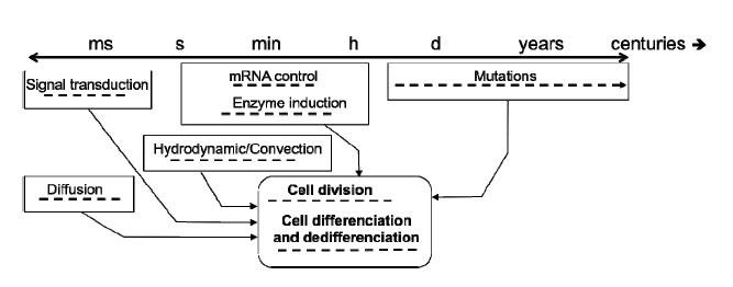
With this global picture in mind, it becomes obvious that describing a cell population at steady state is a specific case study that provides only a partial view of a biosystem. In fact, the phenomena influencing or involved in cell behavior occur under a wide range of characteristic times (Figure 3). It is thus expected that the phenomena with a fast dynamic, which are tedious to observe because of technical limitations in sampling and monitoring, may trigger a change in the long-term cell behavior. Moreover, it is also common to perform studies under the quasi steady state hypothesis, and if the latter is mathematically verified comparing the characteristic times involved, there can be imperceptible underlying physiological changes inducing a strong bias in the conclusions that are drawn.
Therefore, although it is extremely important to identify the steady states a cell is able to maintain when facing varying environmental conditions, it may be useful to characterize how a cell maintains each steady state and how the biosystem evolves within multi steady states. Moreover, it should not be forgotten that at certain steps of any bioprocess (or simply cell culture) the cells will experience transient conditions. In each bioprocess, the early stage of cell culture build-up before the production bioreactor is usually performed in a cascade of bioreactors run in batch mode, which is mostly transient. In the biomedical field, the culture of tissues or cells in regenerative medicine normally involves batch culture mode, and the cells go through highly stressful transient processes when grown onto biomaterials. In a context of producing a biotherapeutic compound, this behavior change may result in a loss in cell productivity. In a biomedical (or medical) context, it may trigger cell differentiation from a desired to a pathological phenotype. MFA and MFBA approaches have proved to be useful for estimating flux distribution in a network at steady and quasi steady state conditions, but dynamic studies (dMFA and dMFBA) are thought to allow for the evaluation of the various impacts of potential dynamic events, as well as enabling MCA studies on a biosystem, characterizing cell behavior under specific perturbations. Therefore, following a system's biology approach, basic knowledge on cell intracellular dynamics and its potential effects on cell metabolism should be integrated. This knowledge, together with the description of the mechanisms involved, will be more than helpful in the development of a descriptive modeling framework that has a predictive capacity.
The usefulness of modeling cell behavior may now be clearer, and we hope that the resulting mathematical model derived from such work will be considered as an invaluable tool to identify innovative solutions in various cases. Such in silico platforms can offer an innovative tool not only for the optimization of bioprocesses, but also in medicine to simulate hypotheses on therapeutics and therapy strategies, as well as in biomedical engineering, for instance, to better understand the problem of losing a desired cell phenotype when using multipotent cells. Although these contexts differ in their research paradigm, the modeling tools developed in each case may be much more similar than might be thought.
Thus, overall, what can we expect from a metabolic model? First, it can definitely contribute to the characterization of a biosystem behavior. However, to be considered as an in silico platform, a model has to demonstrate a predictive capacity. As shown in Figure 2, obtaining a predictive capacity is an ultimate goal, which is expected to be costly in terms of time and effort, as well as financially, taking analytics into account. Nonetheless, such an in silico platform can then help save time and effort and thus accelerate a research project’s success in meeting its objective function(s), such as optimizing a medium composition or fed-batch (or perfusion) culture strategy (i.e. bioreactor control) or identifying “optimal” parental cell lines or robust high-producer clones. As mentioned earlier however the use of a model to identify targets of cell engineering, to test hypotheses on the effect of a therapeutic or a therapy strategy, and to simulate cell differentiation processes may require the contribution of full “omics” technologies.
In fine, it is thought that our capacity to describe the various cell dynamics that affect cell behavior will enable a model’s predictive capacity. However, the question of how important it is to remain close to a biologically relevant description of cell mechanisms while developing mathematical models still remains. The more “biological” a model, the more tedious it could be to statistically validate it with full parameter identification, but this may be the price to pay for a model that could demonstrate a predictive capacity enabling us to explore outside the comfort zone of known experimental conditions, and thus move beyond intuition.
| [1] |
K. Nikodem, On convex stochastic processes, Aequationes Math., 20 (1980), 184–197. doi: 10.1007/BF02190513

|
| [2] |
A. Skowronski, On some properties of j-convex stochastic processes, Aequationes Math., 44 (1992), 249–258. doi: 10.1007/BF01830983
|
| [3] | A. Skowronski, On Wright-convex stochastic processes, Ann. Math. Sil, 9 (1995), 29–32. |
| [4] | Z. Pales, Nonconvex functions and separation by power means, Math. Inequal. Appl., 3 (2000), 169–176. |
| [5] |
D. Kotrys, Hermite-Hadamard inequality for convex stochastic processes, Aequationes Math., 83 (2012), 143–151. doi: 10.1007/s00010-011-0090-1
|
| [6] |
T. Toplu, M. kadakal, I. İşcan, On n-polynomial convexity and some related inequalities, AIMS Math., 5 (2020), 1304–1318. doi: 10.3934/math.2020089
|
| [7] | Z. Brzezniak, T. Zastawniak, Basic stochastic processes: a course through exercises, Springer Science & Business Media, 2000. |
| [8] | K. Sobczyk, Stochastic differential equations with applications to physics and engineering, Springer Science & Business Media, 2013. |
| [9] |
D. Kotrys, Remarks on strongly convex stochastic processes, Aequationes Math., 86 (2013), 91–98. doi: 10.1007/s00010-012-0163-9
|
| [10] | D. Barrez, L. Gonzlez, N. Merentes, A. Moros, On h-convex stochastic processes, Mathematica Aeterna, 5 (2015), 571–581. |
| [11] | M. Shoaib Saleem, M. Ghafoor, H. Zhou, J. Li, Generalization of -convex stochastic processes and some classical inequalities, Math. Probl. Eng., 2020 (2020), 1–9. |
| [12] |
G. Farid, W. Nazeer, M. S. Saleem, S. Mehmood, S. M. Kang, Bounds of Riemann-Liouville fractional integrals in general form via convex functions and their applications, Mathematics, 6 (2018), 248. doi: 10.3390/math6110248
|
| [13] |
S. Zhao, S. I. Butt, W. Nazeer, J. Nasir, M. Umar, Y. Liu, Some Hermiteensenercer type inequalities for k-Caputo-fractional derivatives and related results, Adv. Differ. Equ-NY, 2020 (2020), 1–17. doi: 10.1186/s13662-019-2438-0
|
| [14] | H. Bai, M. S. Saleem, W. Nazeer, M. S. Zahoor, T. Zhao, Hermite-Hadamard-and Jensen-type inequalities for interval nonconvex function, J. Math., 2020 (2020), 1–6. |
| [15] |
S. M. Kang, G. Farid, W. Nazeer, B. Tariq, Hadamard and Fejadamard inequalities for extended generalized fractional integrals involving special functions, J. Inequal. Appl., 2018 (2018), 1–11. doi: 10.1186/s13660-017-1594-6
|
| [16] |
Y. C. Kwun, G. Farid, S. Ullah, W. Nazeer, K. Mahreen, S. M. Kang, Inequalities for a unified integral operator and associated results in fractional calculus, IEEE Access, 7 (2019), 126283–126292. doi: 10.1109/ACCESS.2019.2939166
|
| [17] |
X. Z. Yang, G. Farid, W. Nazeer, Y. M. Chu, C. F. Dong, Fractional generalized Hadamard and Fej-Hadamard inequalities for m-convex function, AIMS Math., 5 (2020), 6325–6340. doi: 10.3934/math.2020407
|
| [18] |
Y. C. Kwun, G. Farid, W. Nazeer, S. Ullah, S. M. Kang, Generalized riemann-liouville -fractional integrals associated with Ostrowski type inequalities and error bounds of hadamard inequalities, IEEE access, 6 (2018), 64946–64953. doi: 10.1109/ACCESS.2018.2878266
|
| [19] |
P. Chen, A. Quarteroni, G. Rozza, Stochastic optimal Robin boundary control problems of advection-dominated elliptic equations, SIAM J. Numer. Anal., 51 (2013), 2700–2722. doi: 10.1137/120884158
|
| [20] |
M. Mnif, H. Pham, Stochastic optimization under constraints, Stoch. Proc. Appl., 93 (2001), 149–180. doi: 10.1016/S0304-4149(00)00089-2
|
| [21] | P. Bank, F. Riedel, Optimal consumption choice under uncertainty with intertemporal substitution, Ann. Appl. Probab., 11 (1999), 788. |
| [22] |
D. Cuoco, Optimal consumption and equilibrium prices with portfolio constraints and stochastic income, J. Econom. Theory, 72 (1997), 33–73. doi: 10.1006/jeth.1996.2207
|
| [23] |
D. Cuoco, J. CvitaniCc, Optimal consumption choice for a large investor, J. Econom. Dyn. Control, 22 (1998), 401–436. doi: 10.1016/S0165-1889(97)00065-1
|
| [24] | J. Cvitanić, I. Karatzas, Convex duality in convex portfolio optimization, Ann. Appl. Probab., 2 (1992), 767–818. |
| [25] | N. El Karoui, M. Jeanblanc, Optimization of consumption with labor income, Financ. Stoch., 4 (1998), 409–440. |
| [26] |
H. He, H. Pagès, Labor income, borrowing constraints and equilibrium asset prices, Economic Theory, 3 (1993), 663–696. doi: 10.1007/BF01210265
|
| [27] |
R. Merton, Optimum consumption and portfolio rules in a continuous-time model, J. Econom. Theory, 3 (1971), 373–413. doi: 10.1016/0022-0531(71)90038-X
|
| [28] |
A. Liu, V. K. Lau, B. Kananian, Stochastic successive convex approximation for non-convex constrained stochastic optimization, IEEE T. Signal Proces., 67 (2019), 4189–4203. doi: 10.1109/TSP.2019.2925601
|
| [29] |
A. Nemirovski, A. Shapiro, Convex approximations of chance constrained programs, SIAM J. Optimiz., 17 (2007), 969–996. doi: 10.1137/050622328
|
| [30] | A. Rakhlin, O. Shamir, K. Sridharan, Making gradient descent optimal for strongly convex stochastic optimization, arXiv preprint arXiv: 1109.5647, 2011. |
| [31] |
S. Ghadimi, G. Lan, Optimal stochastic approximation algorithms for strongly convex stochastic composite optimization i: A generic algorithmic framework, SIAM J. Optimiz., 22 (2012), 1469–1492. doi: 10.1137/110848864
|
| [32] | H. Yu, M. Neely, X. Wei, Online convex optimization with stochastic constraints, Advances in Neural Information Processing Systems, 30 (2017), 1428–1438. |
| [33] | A. Defazio, F. Bach, S. Lacoste-Julien, SAGA: A fast incremental gradient method with support for non-strongly convex composite objectives, Advances in neural information processing systems, 27 (2014), 1646–1654. |
| [34] |
Y. Xu, W. Yin, Block stochastic gradient iteration for convex and nonconvex optimization, SIAM J. Optimiz., 25 (2015), 1686–1716. doi: 10.1137/140983938
|
| [35] | A. K. Sahu, D. Jakovetic, D. Bajovic, S. Kar, Communication-efficient distributed strongly convex stochastic optimization: Non-asymptotic rates, arXiv preprint arXiv: 1809.02920, 2018. |
| [36] | M. Mahdavi, T. Yang, R. Jin, Stochastic convex optimization with multiple objectives, Advances in Neural Information Processing Systems, 26 (2013), 1115–1123. |
| 1. | Yuying Liu, Qi Cao, Wensheng Yang, Influence of Allee effect and delay on dynamical behaviors of a predator–prey system, 2022, 41, 2238-3603, 10.1007/s40314-022-02118-4 | |
| 2. | Chenxuan Nie, Dan Jin, Ruizhi Yang, Hopf bifurcation analysis in a delayed diffusive predator-prey system with nonlocal competition and generalist predator, 2022, 7, 2473-6988, 13344, 10.3934/math.2022737 | |
| 3. | Xiaowen Zhang, Wufei Huang, Jiaxin Ma, Ruizhi Yang, Hopf bifurcation analysis in a delayed diffusive predator-prey system with nonlocal competition and schooling behavior, 2022, 30, 2688-1594, 2510, 10.3934/era.2022128 | |
| 4. | Kuldeep Singh, Mukesh Kumar, Ramu Dubey, Teekam Singh, Untangling role of cooperative hunting among predators and herd behavior in prey with a dynamical systems approach, 2022, 162, 09600779, 112420, 10.1016/j.chaos.2022.112420 | |
| 5. | Xubin Jiao, Li Liu, Xiao Yu, Rich dynamics of a reaction–diffusion Filippov Leslie–Gower predator–prey model with time delay and discontinuous harvesting, 2025, 228, 03784754, 339, 10.1016/j.matcom.2024.09.022 | |
| 6. | Ben Chu, Guangyao Tang, Changcheng Xiang, Binxiang Dai, Dynamic Behaviours and Bifurcation Analysis of a Filippov Ecosystem with Fear Effect, 2023, 2023, 1607-887X, 1, 10.1155/2023/9923003 | |
| 7. | Yunzhuo Zhang, Xuebing Zhang, Shunjie Li, The effect of self-memory-based diffusion on a predator–prey model, 2024, 75, 0044-2275, 10.1007/s00033-024-02256-1 | |
| 8. | Hongyan Sun, Pengmiao Hao, Jianzhi Cao, Dynamics analysis of a diffusive prey-taxis system with memory and maturation delays, 2024, 14173875, 1, 10.14232/ejqtde.2024.1.40 | |
| 9. | Ruying Dou, Chuncheng Wang, Bifurcation analysis of a predator–prey model with memory-based diffusion, 2024, 75, 14681218, 103987, 10.1016/j.nonrwa.2023.103987 | |
| 10. | Yujia Wang, Chuncheng Wang, Dejun Fan, Yuming Chen, Dynamics of a Predator–Prey Model with Memory-Based Diffusion, 2023, 1040-7294, 10.1007/s10884-023-10305-y | |
| 11. | Debasish Bhattacharjee, Dipam Das, Santanu Acharjee, Tarini Kumar Dutta, Two predators, one prey model that integrates the effect of supplementary food resources due to one predator's kleptoparasitism under the possibility of retribution by the other predator, 2024, 10, 24058440, e28940, 10.1016/j.heliyon.2024.e28940 | |
| 12. | L. R. Ibrahim, D. K. Bahlool, Exploring the Role of Hunting Cooperation, and Fear in a Prey-Predator Model with Two Age Stages, 2024, 18, 1823-8343, 727, 10.47836/mjms.18.4.03 | |
| 13. | Li Zou, Zhengdi Zhang, Miao Peng, Stability analysis of an eco-epidemic predator–prey model with Holling type-I and type-III functional responses, 2025, 99, 0973-7111, 10.1007/s12043-024-02877-1 |

Haoliang Fu, Muhammad Shoaib Saleem, Waqas Nazeer, Mamoona Ghafoor, Peigen Li. On Hermite-Hadamard type inequalities for -polynomial convex stochastic processes[J]. AIMS Mathematics, 2021, 6(6): 6322-6339. doi: 10.3934/math.2021371

 DownLoad:
