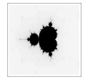
The aim of this paper is to generalize the results regarding fractals and prove escape conditions for general complex polynomial. In this paper we state the orbit of a newly defined iterative scheme and establish the escape criteria in fractal generation for general complex polynomial. We use established escape criteria in algorithms to generate Mandelbrot and Multi-corns sets. In addition, we present some graphs of quadratic, cubic and higher Mandelbrot and Multi-corns sets and discuss how the alteration in parameters make changes in graphs.
Citation: Muhammad Tanveer, Imran Ahmed, Ali Raza, Sumaira Nawaz, Yu-Pei Lv. New escape conditions with general complex polynomial for fractals via new fixed point iteration[J]. AIMS Mathematics, 2021, 6(6): 5563-5580. doi: 10.3934/math.2021329
The aim of this paper is to generalize the results regarding fractals and prove escape conditions for general complex polynomial. In this paper we state the orbit of a newly defined iterative scheme and establish the escape criteria in fractal generation for general complex polynomial. We use established escape criteria in algorithms to generate Mandelbrot and Multi-corns sets. In addition, we present some graphs of quadratic, cubic and higher Mandelbrot and Multi-corns sets and discuss how the alteration in parameters make changes in graphs.

| [1] | B. B. Mandelbrot, The fractal geometry of nature, New York: WH freeman, 1982. |
| [2] |
A. Lakhtakia, V. V. Varadan, R. Messier, V. K. Varadan, On the symmetries of the Julia sets for the process $z\Rightarrow z_p+ c$, J. Phys. A: Math. Gen., 20 (1987), 3533. doi: 10.1088/0305-4470/20/11/051

|
| [3] | B. Branner, The mandelbrot set, Proc. Symp. Appl. Math., 39 (1989), 75–105. |
| [4] | J. W. Milnor, Dynamics in one complex variable: Introductory lectures, Southgate Publishers, 1999. |
| [5] | M. Rani, V. Kumar, Superior julia set, Res. Math. Educ., 8 (2004), 261–277. |
| [6] | M. Rani, V. Kumar, Superior mandelbrot set, Res. Math. Educ., 8 (2004), 279–291. |
| [7] |
X. Zhang, L. Wang, Z. Zhou, Y. Niu, A chaos-based image encryption technique utilizing hilbert curves and H-fractals, IEEE Access, 7 (2019), 74734–74746. doi: 10.1109/ACCESS.2019.2921309
|
| [8] | N. Cohen, Fractal antenna applications in wireless telecommunications, In: Professional Program Proceedings, Electronic Industries Forum of New England, IEEE, 1997. |
| [9] | K. J. Krzysztofik, F. Brambila, Fractals in antennas and metamaterials applications, INTECH Open Sci., Open Minds, Fractal Anal.-Appl. Phys., Eng. Technol., (2017), 45–81. |
| [10] | F. Orsucci, Complexity science, living systems, and reflexing interfaces: New models and perspectives: New models and perspectives, IGI Global, 2012. |
| [11] |
P. Blanchard, R. L. Devaney, A. Garijo, E. D. Russell, A generalized version of the McMullen domain, Int. J. Bifurcation Chaos, 18 (2008), 2309–2318. doi: 10.1142/S0218127408021725
|
| [12] | T. Kim, Quaternion Julia set shape optimization, Comput. Graphics Forum, 34 (2015), 167–176. |
| [13] |
V. Drakopoulos, N. Mimikou, T. Theoharis, An overview of parallel visualisation methods for Mandelbrot and Julia sets, Comput. Graphics, 27 (2003), 635–646. doi: 10.1016/S0097-8493(03)00106-7
|
| [14] |
Y. Sun, L. Chen, R. Xu, R. Kong, An image encryption algorithm utilizing Julia sets and Hilbert curves, PloS one, 9 (2014), e84655. doi: 10.1371/journal.pone.0084655
|
| [15] |
M. Rani, R. Agarwal, Effect of stochastic noise on superior Julia sets, J. Math. Imaging Vision, 36 (2010), 63–68. doi: 10.1007/s10851-009-0171-0
|
| [16] |
M. Rani, R. Chugh, Julia sets and Mandelbrot sets in Noor orbit, Appl. Math. Comput., 228 (2014), 615–631. doi: 10.1016/j.amc.2013.11.077
|
| [17] | S. M. Kang, W. Nazeer, M. Tanveer, A. A. Shahid, New fixed point results for fractal generation in jungck noor orbit with $s$-convexity, J. Funct. Spaces, 2015, (2015). |
| [18] | M. Tanveer, S. M. Kang, W. Nazeer, Y. C. Kwun, New tricorns and multicorns antifractals in Jungck mann orbit, Int. J. Pure Appl. Math., 111 (2016), 287–302. |
| [19] | K. Goyal, B. Prasad, Dynamics of iterative schemes for quadratic polynomial, In: AIP Conference Proceedings, AIP Publishing LLC, 1897 (2017), 020031. |
| [20] | M. Kumari, R. C. Ashish, New Julia and Mandelbrot sets for a new faster iterative process, Int. J. Pure Appl. Math., 107 (2016), 161–177. |
| [21] |
W. Nazeer, S. M. Kang, M. Tanveer, A. A. Shahid, Fixed point results in the generation of Julia and Mandelbrot sets, J. Inequal. Appl., 2015 (2015), 1–16. doi: 10.1186/1029-242X-2015-1
|
| [22] | S. M. Kang, A. Rafiq, A. Latif, A. A. Shahid, Y. C. Kwun, Tricorns and multicorns of-iteration scheme, J. Funct. Spaces, 2015, (2015). |
| [23] |
Y. C. Kwun, M. Tanveer, W. Nazeer, M. Abbas, S. M. Kang, Fractal generation in modified Jungck-S orbit, IEEE Access, 7 (2019), 35060–35071. doi: 10.1109/ACCESS.2019.2904677
|
| [24] |
Y. C. Kwun, M. Tanveer, W. Nazeer, K. Gdawiec, S. M. Kang, Mandelbrot and Julia sets via Jungck-CR iteration with $ s $-convexity, IEEE Access, 7 (2019), 12167–12176. doi: 10.1109/ACCESS.2019.2892013
|
| [25] |
D. Li, M. Tanveer, W. Nazeer, X. Guo, Boundaries of filled julia sets in generalized jungck mann orbit, IEEE Access, 7 (2019), 76859–76867. doi: 10.1109/ACCESS.2019.2920026
|
| [26] |
K. Koyas, S. Gebregiorgis, Coupled coincidence and coupled common fixed points of a pair for mappings satisfying a weakly contraction type $T$-coupling in the context of quasi $ab$-metric space, Open J. Math. Sci., 4 (2020), 369–376. doi: 10.30538/oms2020.0114
|
| [27] |
M. Tesfaye, K. Koyas, S. Gebregiorgis, A coupled fixed point theorem for maps satisfying rational type contractive condition in dislocated quasi $b$-metric space, Open J. Math. Sci., 4 (2020), 27–33. doi: 10.30538/oms2020.0091
|
| [28] | A. Barcellos, Fractals everywhere, by Michael Barnsley, Am. Math. Mon., 97 (1990), 266–268. |
| [29] |
R. L. Devaney, P. B. Siegel, A. J. Mallinckrodt, S. McKay, A first course in chaotic dynamical systems: Theory and experiment, Comput. Phys., 7 (1993), 416–417. doi: 10.1063/1.4823195
|
| [30] |
X. Liu, Z. Zhu, G. Wang, W. Zhu, Composed accelerated escape time algorithm to construct the general Mandelbrot sets, Fractals, 9 (2001), 149–153. doi: 10.1142/S0218348X01000580
|
| [31] | V. V. Strotov, S. A. Smirnov, S. E. Korepanov, A. V. Cherpalkin, Object distance estimation algorithm for real-time fpga-based stereoscopic vision system, In: High-Performance Computing in Geoscience and Remote Sensing VIII, International Society for Optics and Photonics, 2018. |
| [32] | O. Khatib, Real-time obstacle avoidance for manipulators and mobile robots, In: Autonomous robot vehicles, Springer, New York, NY, (1986), 396–404. |
| [33] | J. Barrallo, D. M. Jones, Coloring algorithms for dynamical systems in the complex plane, In: Visual Mathematics, Mathematical Institute SASA, 1999. |


Figures(27)

Muhammad Tanveer, Imran Ahmed, Ali Raza, Sumaira Nawaz, Yu-Pei Lv. New escape conditions with general complex polynomial for fractals via new fixed point iteration[J]. AIMS Mathematics, 2021, 6(6): 5563-5580. doi: 10.3934/math.2021329


 DownLoad: