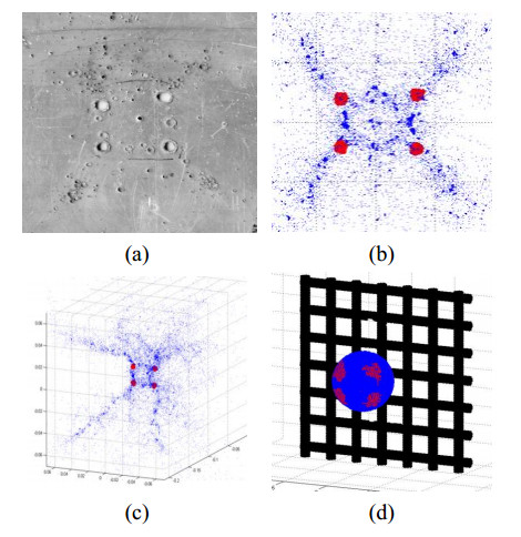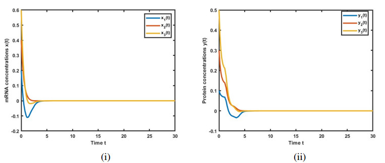
Figure 1.
(i) mRNA concentrations x(t). (ii) Protein concentrations y(t).
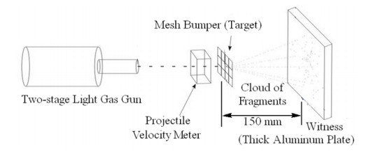
Citation: Nikolay Myagkov, Timofey Shumikhin. Studying the redistribution of kinetic energy between the morphologically distinct parts of the fragments cloud formed from high-velocity impact fragmentation of an aluminum sphere on a steel mesh[J]. AIMS Materials Science, 2019, 6(5): 685-696. doi: 10.3934/matersci.2019.5.685
| [1] | Yajing Zeng, Siyu Yang, Xiongkai Yu, Wenting Lin, Wei Wang, Jijun Tong, Shudong Xia . A multimodal parallel method for left ventricular dysfunction identification based on phonocardiogram and electrocardiogram signals synchronous analysis. Mathematical Biosciences and Engineering, 2022, 19(9): 9612-9635. doi: 10.3934/mbe.2022447 |
| [2] | Jose Guadalupe Beltran-Hernandez, Jose Ruiz-Pinales, Pedro Lopez-Rodriguez, Jose Luis Lopez-Ramirez, Juan Gabriel Avina-Cervantes . Multi-Stroke handwriting character recognition based on sEMG using convolutional-recurrent neural networks. Mathematical Biosciences and Engineering, 2020, 17(5): 5432-5448. doi: 10.3934/mbe.2020293 |
| [3] | Jun Gao, Qian Jiang, Bo Zhou, Daozheng Chen . Convolutional neural networks for computer-aided detection or diagnosis in medical image analysis: An overview. Mathematical Biosciences and Engineering, 2019, 16(6): 6536-6561. doi: 10.3934/mbe.2019326 |
| [4] | Yong Li, Li Feng . Patient multi-relational graph structure learning for diabetes clinical assistant diagnosis. Mathematical Biosciences and Engineering, 2023, 20(5): 8428-8445. doi: 10.3934/mbe.2023369 |
| [5] | Giuseppe Ciaburro . Machine fault detection methods based on machine learning algorithms: A review. Mathematical Biosciences and Engineering, 2022, 19(11): 11453-11490. doi: 10.3934/mbe.2022534 |
| [6] | Eric Ke Wang, Nie Zhe, Yueping Li, Zuodong Liang, Xun Zhang, Juntao Yu, Yunming Ye . A sparse deep learning model for privacy attack on remote sensing images. Mathematical Biosciences and Engineering, 2019, 16(3): 1300-1312. doi: 10.3934/mbe.2019063 |
| [7] | Xu Zhang, Wei Huang, Jing Gao, Dapeng Wang, Changchuan Bai, Zhikui Chen . Deep sparse transfer learning for remote smart tongue diagnosis. Mathematical Biosciences and Engineering, 2021, 18(2): 1169-1186. doi: 10.3934/mbe.2021063 |
| [8] | Long Wen, Liang Gao, Yan Dong, Zheng Zhu . A negative correlation ensemble transfer learning method for fault diagnosis based on convolutional neural network. Mathematical Biosciences and Engineering, 2019, 16(5): 3311-3330. doi: 10.3934/mbe.2019165 |
| [9] | Hui Li, Xintang Liu, Dongbao Jia, Yanyan Chen, Pengfei Hou, Haining Li . Research on chest radiography recognition model based on deep learning. Mathematical Biosciences and Engineering, 2022, 19(11): 11768-11781. doi: 10.3934/mbe.2022548 |
| [10] | Kunli Zhang, Bin Hu, Feijie Zhou, Yu Song, Xu Zhao, Xiyang Huang . Graph-based structural knowledge-aware network for diagnosis assistant. Mathematical Biosciences and Engineering, 2022, 19(10): 10533-10549. doi: 10.3934/mbe.2022492 |
Through their mRNAs, protein expression products, and other components, DNA segments in a cell interact with each other passively, forming dynamic genetic regulatory networks (GRNs) that work as a sophisticated dynamic system to govern biological processes, where the systems of regulatory linkages between DNA, RNA, and proteins comprise GRNs. Modeling genetic networks with dynamical system models, which are a useful tool for analyzing gene regulation mechanisms in living organisms, comes naturally. To examine genetic regulatory developments in life forms, the mathematical models of GRNs comprise formidable tools, which can be approximately separated into two categories, including discrete models [1,2,6,16,22] and continuous models [4,5,9,10,12]. The components in continuous models characterize the concentrations of mRNAs and proteins as continuous data, allowing for a more complete interpretation of GRNs' nonlinear dynamical behavior.
A differential equation is often used to describe a continuous model. Thus, erroneous estimates could result from theoretical models that fail to consider delays. Time delays frequently occur in various applications, and it is widely acknowledged that they can significantly impact system performance, leading to degradation and instability. This realization has sparked significant research interest in the field of stability analysis for systems with time delays over recent years, such as differential equations [35], neural networks [11,13,24], bidirectional associative memory fuzzy neural networks [36], fuzzy competitive neural networks [37], and neutral-type neural networks [14,25,27]. More accurate descriptions of GRNs are possible using differential equation models with delayed states, also called delayed GRNs, which offer a better display of the nature of life. To indicate the time needed for transcription, translation, phosphorylation, protein degradation, translocation, and posttranslational modification, time delays are often established in cellular models. Particularly for eukaryotes, delays may affect the firmness and dynamics of the whole system considerably. While there are limited quantitative assessments of the delays, developments in quantifying RNA splicing delays should be taken into account. Because the time delays in biochemical reactions align with or surpass other important time scales defining the cellular system, and the feedback loops related to these delays are robust, and these delays become pivotal for explaining transient processes. This suggests that in cases where delay durations are substantial, both analytical and numerical modeling need to consider the impact of time delays, which has led to the study of various stability forms of the system, for example, in [5,10,31,33,38]. A common type of time delay, referred to as leakage delay (i.e., the delay associated with leaking or forgetting items) might arise within the negative feedback components of networks and has a substantial impact on the dynamics, potentially resulting in instability or suboptimal performance in GRNs. In fact, various beneficial algorithms and computational tools have been devised to address this phenomenon, with numerous notable findings published in previous literature [7,17,28,29,32].
When a built system has been implemented in the field, there is typically some unpredictability; be it a windy sky or a rough road, we may encounter uncertainty in the operational area. Uncertainty can also be found in the system's defining variables, such as torque constants and physical dimensions. As a consequence of the dynamic nature of a system under investigation, one of the most critical attributes of that system is stability. In general, when a system is chaotic, or simply lacks stability, it is not especially useful. It is preferable to work with systems that are stable or offer periodic behavior, with the caveat that chaotic behavior can be readily understood in some systems, and there can also sometimes be good reasons for people to actively seek chaos in a system for various applications. Therefore, we found research that demonstrated various stability criteria such as asymptotic stability analysis, exponential stability analysis [3,34], H infinity performance [25], finite-time stability (FTS) analysis [15,23], and so on. The concept of FTS differs from classical stability in two significant ways. First, it addresses systems whose functionality is limited to a fixed finite time interval. Second, FTS necessitates predefined constraints on system variables. This is particularly relevant for systems that are recognized to operate exclusively within a finite time span and in cases where practical considerations dictate that system variables must adhere to specific bounds[8].
After thorough investigation, FTS for GRNs with delays has been studied in references [21,24,26], as well as [39]. For example, the researchers in reference [21] explored the FTS for GRNs that have demonstrated impulsive effects, employing the Lyapunov function method. In [24], the topic of FTS for switched GRNs with time-varying delays was examined through the use of Wirtinger's integral inequality. Furthermore, the effect of leakage delay has been studied in various works, including references [14,18,27]. For instance, in [14], the researchers proposed sufficient conditions that guarantee the asymptotic stability of GRNs, which have a neutral delay and are affected by leakage delay through the application of the Lyapunov functional. Additionally, in reference [18], the authors focused on global asymptotic stability analysis aimed at stabilizing switched stochastic GRNs that exhibit both leakage and impulsive effects. This stabilization has depended on both time-varying delay and distributed time-varying delay terms, utilizing contemporary Lyapunov-Krasovskii functional and integral inequality techniques. However, it has been determined that there are no studies focusing on analyzing the FTS while considering the effect of leakage delay for GRNs. The successful completion of such research could contribute to a deeper comprehension of leakage delay and potentially offer opportunities to improve the stability criteria of GRNs. This research concerns the effect of the leakage delays on FTS criteria for GRNs with interval time-varying delays. The criteria aim to consider the effect of leakage delays. Consequently, we employ the construction of a Lyapunov-Krasovskii (LK) function and estimate various integral inequalities as well as reciprocally convex techniques to establish them. These improvements enable us to specify the stability criteria concerning the effect of leakage delays on FTS. This refinement simplifies the representation of stability criteria in the form of linear matrix inequalities (LMIs). Ultimately, we offer a numerical example to demonstrate the effect of leakage delays and emphasize the significance of our theoretical findings.
The principal contributions of this research can be encapsulated as follows:
(i) Targeted focus on leakage delays: We specifically address the impact of leakage delays on the finite-time stability of GRNs, filling a gap in existing research and providing new data on the stability dynamics influenced by these delays.
(ii) Consideration of variable delay limits: We take into account the lower limits on delays, which can vary between positive values and zero, and accommodate the derivatives of delays ranging from negative to positive. This comprehensive approach allows for the one that offers a better representation of the nature of organism and modeling of real biological scenarios.
(iii) Empirical validation: A numerical example is provided to demonstrate the implications of leakage delays on the stability criteria. This example underscores the impact of leaked delays on GNRs.
(iv) Contribution to broader fields: The insights gained from this study have the potential to advance multiple fields, including systems biology, biotechnology, and medicine.
By addressing these aspects, this research significantly enhances our understanding of the interplay between leakage delays and finite-time stability in genetic regulatory networks, paving the way for future studies and applications in various scientific and medical domains.
The first step is to introduce the following symbols or notations: Rn and Rn×r represent the n-dimensional Euclidean space and the set of all n×r real matrices, respectively; G>0 (G≥0) signifies that the symmetric matrix G is positive (semi-positive) definite; G<0 (G≤0) signifies that the symmetric matrix G is negative (semi-negative) definite; The quadratic from ‖φ(t)‖2N is defined as: ‖φ(t)‖2N=φT(t)Nφ(t) or ‖φ(t)‖N=√φT(t)Nφ(t) for any state vector φ(t), and N≥0.
In this paper, we suggest the GRNs with interval time-varying delays and leakage delays in the form
| ˙mi(t)=−aimi(t−ρa)+∑nj=1wijgj(pj(t−r(t)))+ϵi,˙pi(t)=−cipi(t−ρc)+dimi(t−h(t)),i=1,2,…,n, | (2.1) |
where mi(⋅) and pi(⋅) are the concentrations of mRNA and protein of the ith node at time t, respectively. ai>0 and ci>0 denotes the degradation or dilution rates of mRNAs and proteins, retrospectively. di represents the translation. wij is defined as follows:
| wij={γijif transcription factor j is an activator of gene i;0if there is no link from node j to i;−γijif transcription factor j is an repressor of gene i. |
r(⋅) and h(⋅) are the feedback regulation and translation delays, respectively, which are retrospectively satisfied by
| 0<rm≤r(t)≤rM,rdm≤˙r(t)≤rdM, | (2.2) |
| 0<hm≤h(t)≤hMhdm≤˙h(t)≤hdM, | (2.3) |
where ρa>0 and ρc>0 denote the leakage delays. gj(pj(s))=(pj(s)/Bj)Hj/(1+pj/Bj)Hj where Hj is the monotonic function in Hill form, ϵi=∑j∈Ukγij with Uk={j| the jth transcription factor being a repressor of the kth gene, j=1,…,n}, Bj>0 is a constant which the feedback regulation of the protein on the transcription. When we let (m∗,p∗)T be an equilibrium point of (2.1), the equilibrium point can be shifted to the origin by transformation: xi(t)=mi−m∗i,yi(t)=pi−p∗i, and system (2.1) can be rewritten in the vector form
| ˙x(t)=−Ax(t−ρa)+Wf(y(t−r(t))),˙y(t)=−Cy(t−ρc)+Dx(t−h(t)),x(t)=ϕ(t),y(t)=ξ(t),t∈[−τ,0],τ=max{hM,rM,ρa,ρc}, | (2.4) |
where A=diag(a1,a2,...,an), C=diag(c1,c2,...,cn), W=[wij]n×n, f(y(t))=g(y(t))−p∗ with f(0)=0, ϕ(t),t∈[−max{ρa,hM},0] and ξ(t),t∈[−max{ρc,rM},0] are the initial conditions.
Assumption 1. The regulatory function f(ζ(t))=[f1(ζ1(t)),f2(ζ2(t)),...,fn(ζn(t))]T∈Rn is assumed to satisfy the following condition
| ℘−i≤fi(ζ1)−fi(ζ2)ζ1−ζ2≤℘+i,f(0)=0,ζ1,ζ2∈R,ζ1≠ζ2,i=1,2,...,n, | (2.5) |
where ℘−i,℘+i are real constants, and let ð−=diag(℘−1,℘−2,…,℘−n), ð+=diag(℘+1,℘+2,…,℘+n) and ℘i=diag(max{|℘−j|,|℘+j|}), ð=diag(℘1,℘2,…,℘n).
Then, the definition presented along with the several lemmas serves as a methodologies utilized to prove our primary outcomes.
Definition 2.1. (see [21]) Let G≥0 be a matrix, if
| ‖Φ(t)‖2G+‖Ψ(t)‖2G≤c1→‖x(t)‖2G+‖y‖2G≤c2,∀t∈[0,T], |
where ‖Φ(t)‖G=sup−max{ρa,hM}≤t≤0{‖ϕ(t)‖G,‖˙ϕ(t)‖G} and ‖Ψ(t)‖G=sup−max{ρc,rM}≤t≤0{‖ξ(t)‖G,‖˙ξ(t)‖G}, then the GRNs with interval time-vary delays and leakage delays (2.4) exhibits FTS concerning positive real numbers (c1,c2,T).
Lemma 2.2. Let N∈Rn×n, N=NT>0 and G∈Rn×n,G=GT be any constant matrices. Then
| λmin(N−1G)φTNφ≤φTGφ≤λmax(N−1G)φTNφ, |
where the expressions "λmin(N−1G)" and "λmax(N−1G)" denote the minimum real part and the maximum real part of the eigenvalues of N−1G respectively.
Lemma 2.3. (Jensen's inequality [28]). Let G∈Rn×n, G=GT>0 be any constant matrix, δM be positive real constant and φ:[−δM,0]→Rn be vector-valued function. Then,
| −δM∫tt−δMφT(s)Gφ(s)ds≤−∫tt−δMφT(s)dsG∫tt−δMφ(s)ds. |
Lemma 2.4 (see [30]). Let G∈Rn×n, G=GT>0 be any constant matrix, δm>0,δM>0 are real constants and φ:[−δM,−δm,]→Rn be vector-valued function. Then,
| −(δM−δm)∫t−δmt−δMφT(s)Gφ(s)ds≤−∫t−δmt−δMφT(s)dsG∫t−δmt−δMφ(s)ds. |
Lemma 2.5 (see [20]). Let G∈Rn×n, G=GT>0 be any constant matrix, and any continuously differentiable function z:[δm,δM]→Rn. Then,
| (δM−δm)∫δMδmφT(s)Gφ(s)ds≥ℵT1Gℵ1+3ℵT2Gℵ2,(δM−δm)∫δMδm˙φT(s)G˙φ(s)ds≥ℵT3Gℵ3+3ℵT4Gℵ4+5ℵT5Gℵ5, |
where
| ℵ1=∫δMδmφ(s)ds,ℵ2=∫δMδmφ(s)ds−2δM−δm∫δMδm∫δMθφ(s)dsdθ,ℵ3=φ(δM)−φ(δm),ℵ4=φ(δM)+φ(δm)−2δM−δm∫δMδmφ(s)ds,ℵ5=φ(δM)−φ(δm)+6δM−δm∫δMδmφ(s)ds−12(δM−δm)2∫δMδm∫δMθφ(s)dsdθ. |
Lemma 2.6. (see [19]). Let κ1,κ2,…,κN:Rn→R have positive values in an open subset D of Rn. Then, the reciprocally convex combination of κi over D satisfies
| min{αi|α1>0,∑iαi=1}∑i1αiκi(t)=∑iκi(t)+maxηi,j(t)∑i≠jηi,j(t), |
subject to
| {ηi,j:Rn⇒R,ηi,j=ηj,i,[κi(t)ηi,j(t)ηj,i(t)κj(t)]≥0}. |
Lemma 2.7. (see [11,13]). Suppose Assumption 1 is valid, let diagonal matrices Γi>0,i=1,2. Then
| [ζ(t)f(ζ(t))]T[−Γ1Ξ1Γ1Ξ2Γ1Ξ2−Γ1][ζ(t)f(ζ(t))]≥0, | (2.6) |
| [ζ(t−r(t))f(ζ(t−r(t)))]T[−Γ2Ξ1Γ2Ξ2Γ2Ξ2−Γ2][ζ(t−r(t))f(ζ(t−r(t)))]≥0, | (2.7) |
where Ξ1=diag(℘−1℘+1,℘−2℘+2,…,℘−n℘+n) and Ξ2=diag(℘−1+℘+12,℘−2+℘+22,…,℘−n+℘+n2).
In this section, we present a theorem and a corollary related to GRNs. To begin with, the FTS result is formulated for the GRNs with interval time-varying delays, considering the effect of leakage delays.
Theorem 3.1. Given that Assumption 1 valid. For positive scalars c1,c2,T,α, ρa, ρc, hm, hM, hdm, hdM, rm, rM, rdm and rdM according conditions (2.2)–(2.3), if there exist matrices Pi>0,i=1,2,3, Qi>0,i=1,2,3,4, Ri>0,i=1,2, Si>0,i=1,2,3,4, Ui>0,i=1,2, any diagonal matrices Γi>0,i=1,2, any appropriate dimensional matrices Ei,Ni,i=1,2,3,4, satisfying the following conditions:
| [S2X1i∗S2]≥0,i=1,2,3,[S4X2i∗S4]≥0,,i=1,2,3,Θ<0, | (3.1) |
| λ1λ2eαTc1≤c2. | (3.2) |
Then, the system (2.4) exhibits FTS concerning N>0 and positive real numbers (c1,c2,T), where Θ=∑7i=1Θi is defined as
| Θ1=2[e1e5]T[P1ET10ET2][e5−e5−A(e1−e13)+We8]+eT1P2e1−eαhmeT2P2e2+eαhmeT2P3e2+(hdMeαhM−eαhm)eT3P3e3+(eαhM−hdmeαhm)eT3P3e3−eαhMeT4P3e4−αeT1P1e1,Θ2=2[e6e10]T[P3ET30ET4][e10−e10−C(e6−e14)+De3]+eT6Q2e6−eαrmeT7Q2e7+eαhmeT7Q3e7+(rdMeαrM−eαrm)eT8Q3e8+(eαrM−rdmeαrm)eT9Q3e9−eαrmeT9Q3e9+eT11Q4e11+(rdMeαrM−eαrm)eT12Q4e12−αeT6Q1e6,Θ3=h2MeT1R1e1+r2MeT6R2e6−ℵT11(h2mR1)ℵ11−3ℵT12(h2mR1)ℵ12−ℵT21(r2mR2)ℵ21−3ℵT22(r2mR2)ℵ22,Θ4=eT5(h2mS1+h2MmS2)e5+eT10(r2mS3+r2MmS4)e10−ℵT31S1ℵ31−3ℵT41S1ℵ41−5ℵT51S1ℵ51−ℵT32S3ℵ32−3ℵT42S3ℵ42−5ℵT52S3ℵ52+eαhm(−ℵT61Qℵ61−3ℵT71Qℵ71−5ℵT81Qℵ81−ℵT62Qℵ62−3ℵT72Qℵ72−5ℵT82Qℵ82)+eαrm(−ℵT91Qℵ91−3ℵT101Qℵ101−5ℵT111Qℵ111−ℵT92Qℵ92−3ℵT102Qℵ102−5ℵT112Qℵ112)+2eαhm(−ℵT61X11ℵ62−3ℵT71X12ℵ72−5ℵT81X13ℵ82)+2eαrm(−ℵT91X21ℵ92−3ℵT101X22ℵ102−5ℵT111X23ℵ112),Θ5=ρ2aeT5U1e5+ρ2ceT10U2e10−eT13U1e13−eT14U2e14,Θ6=2[e6e11]T[−Γ1Ξ1Γ1Ξ2Γ1Ξ2−Γ1][e6e11]+2[e8e12]T[−Γ2Ξ1Γ2Ξ2Γ2Ξ2−Γ2][e8e12],Θ7=2(e1−e3−e21)TM1(−C(e6−e14)+De3−e10)T+2(e1−e3−e21)TM2e1+2(e1−e3−e21)TM3e3+2(e1−e3−e21)TM4e21,ℵ11=1hme15,ℵ12=1hm(e15−2e22),ℵ21=1rme16,ℵ22=1rm(e16−2e23),ℵ31=e1−e2,ℵ41=e1+e2−2e15,ℵ51=e1−e2+6e15−12e22,ℵ32=e6−e7,ℵ42=e6+e7−2e16,ℵ52=e6−e7+6e16−12e23,ℵ61=e2−e3,ℵ71=e2+e3−2e17,ℵ81=e2−e3+6e17−12e24,ℵ62=e3−e4,ℵ72=e3+e4−2e18,ℵ82=e3−e4+6e18−12e25,ℵ91=e7−e8,ℵ101=e7+e8−2e19,ℵ111=e7−e8+6e19−12e26,ℵ92=e8−e9,ℵ102=e8+e9−2e20,ℵ112=e8−e9+6e20−12e27,hMm=hM−hm,rMm=rM−rm,β1h=eαhm−1α,β2h=eαhM−eαhmα,β3h=eαhm−αhm−1α2β4h=eαhM−eαhm+α(hm−hM)α2,β1r=eαrm−1α,β2r=eαrM−eαrmα,β3r=eαrM−1α,β4r=eαrm−αrm−1α2,β5r=eαrM−eαrm+α(rm−rM)α2,β1ρ=eαρa−1α,,β2ρ=eαρc−1α,ej=[0n×(j−1)nIn0n×(j−14)n],j=1,2,…,27. |
Proof. First, we employ the Newton-Leibniz formula to modify system (2.4), which is as follows
| ˙x(t)=−A(x(t)−∫tt−ρa˙x(s)ds)+Wf(y(t−r(t))),˙y(t)=−C(y(t)−∫tt−ρc˙y(s)ds)+Dx(t−h(t)). | (3.3) |
Second, the LK functional is designed for the system (3.3) :
| V(t)=5∑i=1Vi(t), | (3.4) |
where
| V1(t)=xT(t)P1x(t)+∫tt−hmeα(t−s)xT(s)P2x(s)ds+∫t−hmt−hMeα(t−s)xT(s)P3x(s)ds,V2(t)=yT(t)Q1y(t)+∫tt−rmeα(t−s)yT(s)Q2y(s)ds+∫t−rmt−rMeα(t−s)yT(s)Q3y(s)ds,+∫tt−r(t)eα(t−s)fT(y(s))Q4f(y(s))dsV3(t)=hm∫0−hm∫tt+θeα(t−s)xT(s)R1x(s)dsdθ+rm∫0−rm∫tt+θeα(t−s)yT(s)R2y(s)dsdθ,V4(t)=hm∫0−hm∫tt+θeα(t−s)˙xT(s)S1˙x(s)dsdθ+hMm∫−hm−hM∫tt+θeα(t−s)˙xT(s)S2˙x(s)dsdθ+rm∫0−rm∫tt+θeα(t−s)˙yT(s)S3˙y(s)dsdθ+rMm∫−rm−rM∫tt+θeα(t−s)˙yT(s)S4˙y(s)dsdθ,V5(t)=ρa∫0−ρa∫tt+θeα(t−s)˙xT(s)U1˙x(s)dsdθ+ρc∫0−ρc∫tt+θeα(t−s)˙yT(s)U2˙y(s)dsdθ. |
Then, taking ˙Vi(t) along the trajectory of system (3.3) with (2.2) and (2.3), we have
| ˙V1(t)=2xT(t)P1˙x(t)+xT(t)P2x(t)−eαhmxT(t−hm)P2x(t−hm)+eαhmx(t−hm)P3x(t−hm)−(1−˙h(t))eαh(t)xT(t−h(t))P3x(t−h(t))+(1−˙h(t))eαh(t)xT(t−h(t))P3x(t−h(t))−eαhMxT(t−hM)P3x(t−hM)−αxT(t)P1x(t)+αV1(t). |
Utilizing the zero equation −˙x(t)−A(x(t)−∫tt−ρa˙x(s)ds)+Wf(y(t−r(t)))=0, we estimate the boundary hdm≤˙h(t)≤hdM, and the exponential function term 1=e0≤eαhm≤eαh(t)≤eαhM, −1=−e0≥−eαhm≥−eαh(t)≤−eαhM. From this, we derive the values of ˙V1(t) as follows.
| ˙V1(t)≤2[x(t)˙x(t)]T[P1ET10ET2][˙x(t)−˙x(t)−A(x(t)−∫tt−ρa˙x(s)ds)+Wf(y(t−r(t)))]+xT(t)P2x(t)−eαhmxT(t−hm)P2x(t−hm)+eαhmxT(t−hm)P3x(t−hm)+(hdMeαhM−eαhm)×xT(t−h(t))P3x(t−h(t))+(eαhM−hdmeαhm)xT(t−h(t))P3x(t−h(t))−eαhMxT(t−hM)P3x(t−hM)−αxT(t)P1x(t)+αV1(t)≤χT(t)Θ1χ(t)+αV1(t). |
Using the same method, the zero equation as −˙y(t)−C(y(t)−∫tt−ρc˙y(s)ds)+Dx(t−h(t)))=0 allows us to obtain the derivative of V2(t), which is
| ˙V2(t)≤2[y(t)˙y(t)]T[Q1ET30ET4][˙y(t)−˙y(t)−C(y(t)−∫tt−ρc˙y(s)ds)+Dx(t−h(t)))]T+yT(t)Q2y(t)−eαrmyT(t−rm)Q2y(t−rm)+eαrmyT(t−rm)Q3y(t−rm)+(rdMeαrM−eαrm)×y(t−r(t))Q3y(t−r(t))+(eαrM−rdmeαrm)y(t−r(t))Q3y(t−r(t)))−eαrMyT(t−rM)Q3y(t−rM)+fT(y(t))Q4f(y(t))+(rdMeαrM−eαrm)fT(y(t−r(t)))×Q4f(y(t−r(t)))−αyT(t)Q1y(t)+αV2(t)≤χT(t)Θ2χ(t)+αV2(t). |
The derivative of V3(t) is calculated to obtain
| ˙V3(t)≤xT(t)(h2mR1)x(t)+yT(t)(r2mR2)y(t)−hm∫tt−hmxT(s)Q1x(s)ds−rm∫tt−rmyT(s)Q3y(s)ds+αV3(t). |
We utilize Lemma 2.5 to estimate the amount, leading to the subsequent inequality.
| ˙V3(t)≤χT(t)(eT1(h2mR1)eT1+eT6(r2mR2)e6−ℵT11(h2mR1)ℵ11−3ℵT12(h2mR1)ℵ12−ℵT21Q(r2mR2)ℵ21−3ℵT22(r2mR2)ℵ22)χ(t)+αV3(t)=χT(t)Θ3χ(t)+αV3(t). | (3.5) |
The derivative of V4(t) is calculated to obtain
| ˙V4(t)=˙xT(t)(h2mS1+h2MmeαhmS2)˙x(t)+˙yT(t)(r2mS3+r2MmeαrmS4)˙y(t)−hm∫tt−hm˙xT(s)S1˙x(s)ds−rm∫tt−rm˙yT(s)S3˙y(s)ds−hMmeαhm∫t−hmt−hM˙xT(s)S2˙x(s)ds−rMmeαrm∫t−rmt−rM˙yT(s)S4˙y(s)ds+αV3(t). |
To facilitate our analysis, we decompose and examine the inequality in the derivative of V4(t) step by step as follows. In the first part, we use Lemma 2.5 to approximate the value, resulting in the following inequality.
| −hm∫tt−hm˙xT(s)S1˙x(s)ds−rm∫tt−rm˙yT(s)S3˙y(s)ds≤χT(t)(−ℵT31S1ℵ31−3ℵT41S1ℵ41−5ℵT51S1ℵ51−ℵT32S3ℵ32−3ℵT42S3ℵ42−5ℵT52S3ℵ52)χ(t). | (3.6) |
Then, we estimate the values of the second part of the inequality as follows.
| −hMmeαhm∫t−hmt−hM˙xT(s)S2˙x(s)ds−rMmeαrm∫t−rmt−rM˙yT(s)S4˙y(s)ds=−hMmeαhm(h(t)−hm)(h(t)−hm)∫t−hmt−h(t)˙xT(s)S2˙x(s)ds−hMmeαhm(hM−h(t))(hM−h(t))∫t−h(t)t−hM˙xT(s)S2˙x(s)ds−rMmeαrm(r(t)−rm)(r(t)−rm)∫t−rmt−r(t)˙yT(s)S4˙y(s)ds−rMmeαrm(rM−r(t))(rM−r(t))∫t−r(t)t−rM˙yT(s)S4˙y(s)ds. |
By utilizing Lemma 2.5 together with Lemma 2.6, we can approximate the inequality as follows
| −hMmeαhm∫t−hmt−hM˙xT(s)Q2˙x(s)ds−rMmeαrm∫t−rmt−rM˙yT(s)Q4˙y(s)ds≤χT(t)(eαhm(−ℵT61Qℵ61−3ℵT71Qℵ71−5ℵT81Qℵ81−ℵT62Qℵ62−3ℵT72Qℵ72−5ℵT82Qℵ82)+eαrm(−ℵT91Qℵ91−3ℵT101Qℵ101−5ℵT111Qℵ111−ℵT92Qℵ92−3ℵT102Qℵ102−5ℵT112Qℵ112)+2eαhm(−ℵT61X11ℵ62−3ℵT71X12ℵ72−5ℵT81X13ℵ82)+2eαrm(−ℵT91X21ℵ92−3ℵT101X22ℵ102−5ℵT111X23ℵ112))χ(t). | (3.7) |
Estimating the derivatives of V4(t) along with approximating the values, in inequalities (3.6) and (3.7) is a crucial part of this analysis. We obtained consistent equations in this process as follows:
| ˙V4(t)≤χT(t)Θ4χ(t)+αV4(t). | (3.8) |
Regarding V5(t), we derived its derivative and applied Lemma 2.4 for estimation. Additionally, when approximating the exponential function where 1=e0≤eαρa, 1=e0≤eαρc, −1=−e0≥−eαρa, −1=−e0≥−eαρc, we obtain the following results
| ˙V5(t)≤ρ2a˙xT(t)U1˙x(t)+ρ2c˙yT(s)U2˙y(t)−∫tt−ρa˙xT(s)dsU1∫tt−ρa˙x(s)ds−∫tt−ρc˙yT(s)dsU2∫tt−ρc˙y(s)ds+αV5(t)=χT(t)Θ5χ(t)+αV5(t). | (3.9) |
Next, by adopting Eqs (2.6) and (2.7) and let Γi>0,i=1,2 be diagonal matrices, we obtain
| [y(t)f(y(t))]T[−Γ1Ξ1Γ1Ξ2Γ1Ξ2−Γ1][y(t)f(y(t))]+[y(t−r(t))f(y(t−r(t)))]T[−Γ2Ξ1Γ2Ξ2Γ2Ξ2−Γ2][y(t−r(t))f(y(t−r(t)))]=χT(t)Θ6χ(t)>0. |
Additionally, we utilize the zero equation derived from the Newton-Leibniz equation: x(t)−x(t−h(t))−∫tt−h(t)˙x(s)ds=0. Let Ni,i=1,2,3,4 be appropriate dimensional matrices, resulting in the equation:
| χT(t)(2(e1−e3−e21)TM1(−C(e6−e14)+De3−e10)T+2(e1−e3−e21)TM2e1+2(e1−e3−e21)TM3e3+2(e1−e3−e21)TM4e21)χ(t)=χT(t)Θ7χ(t)=0. | (3.10) |
It becomes evident that, upon estimating ˙V(t) after recalling (3.1), we receive
| ˙V(t)−αV(t)≤0, | (3.11) |
where ˙V(t)≤χT(t)Θχ(t)+αV(t), χT(t)=[xT(t),xT(t−hm),xT(t−h(t)),xT(t−hM),˙xT(t),yT(t),yT(t−rm),yT(t−r(t)),yT(t−rM), ˙yT(t),fT(y(t)),fT(y(t−r(t))),∫tt−ρa˙xT(s)ds,∫tt−ρc˙yT(s)ds,1hm∫tt−hmxT(s)ds,1rm∫tt−rmyT(s)ds, 1h(t)−hm∫t−hmt−h(t)xT(s)ds,1hM−h(t)∫t−h(t)t−hMxT(s)ds,1r(t)−rm∫t−rmt−r(t)yT(s)ds,1rM−r(t)∫t−r(t)t−rMyT(s)ds,∫tt−h(t)˙xT(s)ds, 1h2m∫tt−hm∫tθxT(s)dsdθ,1r2m∫tt−rm∫tθyT(s)dsdθ,1(h(t)−hm)2∫t−hmt−h(t)∫t−hmθxT(s)dsdθ,1(hM−h(t))2∫t−h(t)t−hM ×∫t−h(t)θxT(s)dsdθ,1(r(t)−rm)2∫t−rmt−r(t)∫t−rmθyT(s)dsdθ,1(rM−r(t))2∫t−r(t)t−rM∫t−r(t)θyT(s)dsdθ].
By multiplying the inequality (3.11) by e−αt and integrating from 0 to t where t belongs to the interval [0,T], we derive the following result:
| V(t)≤eαtV(0), |
where
| V(ϕ(0),ξ(0))=ϕT(0)P1ϕ(0)+∫0−hme−αsϕT(s)P2ϕ(s)ds+∫−hm−hMe−αsϕT(s)P3ϕ(s)ds+ξT(0)Q1ξ(0)+∫0−rme−αsξT(s)Q2ξ(s)ds+∫−rm−rMe−αsξT(s)Q3ξ(s)ds+∫0−r(0)e−αsfT(ξ(s))Q4f(ξ(s))ds+hm∫0−hm∫0θe−αsϕT(s)R1ϕ(s)dsdθ+rm∫0−rm∫0θe−αsξT(s)R2ξ(s)dsdθ+hm∫0−hm∫0θe−αs˙ϕT(s)S1˙ϕ(s)dsdθ+hMm∫−hm−hM∫0θe−α−s˙ϕT(s)S2˙ϕ(s)dsdθ+rm∫0−rm∫0θe−αs˙ξT(s)S3˙ξ(s)dsdθ+rMm∫−rm−rM∫0θe−αs˙ξT(s)S4˙ξ(s)dsdθ+ρa∫0−ρa∫0θe−αs˙ϕT(s)U1˙ϕ(s)dsdθ+ρc∫0−ρc∫0θe−αs˙ξT(s)U2˙ξ(s)dsdθ |
| ≤λmax(N−1P1)ϕT(0)NϕT(0)+∫0−hme−αsλmax(N−1P2)ϕT(s)Nϕ(s)ds+∫−hm−hMe−αsλmax(N−1P3)×ϕT(s)Nϕ(s)ds+λmax(N−1Q1)ξT(0)Nξ(0)+∫0−rme−αsλmax(N−1Q2)ξT(s)Nξ(s)ds+∫−rm−rMe−αsλmax(N−1Q3)ξT(s)Nξ(s)ds+∫0−r(0)e−αsλmax(N−1Q4)fT(ξ(s))Nf(ξ(s))ds+hm∫0−hm∫0θe−αsλmax(N−1R1)ϕT(s)Nϕ(s)dsdθ+rm∫0−rm∫0θe−αsλmax(N−1R2)ξT(s)Nξ(s)dsdθ+hm∫0−hm∫0θe−αsλmax(N−1S1)˙ϕT(s)N˙ϕ(s)dsdθ+hMm∫−hm−hM∫0θe−αsλmax(N−1S2)˙ϕT(s)N˙ϕ(s)dsdθ+rm∫0−rm∫0θe−αsλmax(N−1S3)˙ξT(s)N˙ξ(s)dsdθ+rMm∫−rm−rM∫0θe−αsλmax(N−1S4)˙ξT(s)N˙ξ(s)dsdθ+ρa∫0−ρa∫0θe−αsλmax(N−1U1)˙ϕT(s)N˙ϕ(s)dsdθ+ρc∫0−ρc∫0θe−αsλmax(N−1U2)˙ξT(s)N˙ξ(s)dsdθ≤λmax(N−1P1)‖ϕ(t)‖2N+β1hλmax(N−1P2)‖ϕ(t)‖2N+β2hλmax(N−1P3)‖ϕ(t)‖2N+λmax(N−1Q1)‖ξ(t)‖2N+β1rλmax(N−1Q2)‖ξ(s)‖2N+β2rλmax(N−1Q3)‖ξ(t)‖2N+β3rλmax(N−1Q4)λmax(ðTð)‖ξ(t)‖2N+β3hλmax(N−1R1)‖ϕ(t)‖2N+β4rλmax(N−1R2)‖ϕ(t)‖2N+β3hλmax(N−1S1)‖ξ(t)‖2N+β4rλmax(N−1S2)‖ξ(t)‖2N+β4hλmax(N−1S3)‖ϕ‖2N+β5rλmax(N−1S4)‖ξ‖2N+β1ρλmax(N−1U1)‖ϕ(t)‖2N+β2ρλmax(N−1U2)‖ξ(s)‖2N≤λ1(‖Φ(t)‖2N+‖Ψ(t)‖2N), | (3.12) |
where ‖Φ(t)‖N=sup−max{ρ1,hM}≤t≤0{‖ϕ(t)‖N,‖˙ϕ(t)‖N} and ‖Ψ(t)‖N=sup−max{ρ2,rM}≤t≤0{‖ξ(t)‖N,‖˙ξ(t)‖N}, λ1=λmax((N−1P1)+β1h(N−1P2)+β2h(N−1P3)+(N−1Q1)+β1r(N−1Q2)+β2r(N−1Q3)+β3r(N−1Q4)(ðTð)+β3h(N−1R1)+β4r(N−1R2)+β3h(N−1S1)+β4r(N−1S2)+β4h(N−1S3)+β5r(N−1S4)+β1ρ(N−1U1)+β2ρ(N−1U2)), and N>0.
In the interim,
| V(t)≥min{λmin(P1N−1)‖x(t)‖2N+λmin(Q1N−1)‖y(t)‖2N}≥λ2(‖x(t)‖2N+‖y(t)‖2N), | (3.13) |
where λ2=λmin(N−1P1+N−1Q1). Let c1 be a positive real number where
| ‖Φ(t)‖2N+‖Ψ(t)‖2N≤c1. |
Combining inequalities (3.11)–(3.13) we acquire:
| (‖x(t)‖2N+‖y(t)‖2N)≤1λ2eαTV(ϕ(0),ξ(0))≤1λ2eαTλ1c1≤λ1λ2eαTc1≤c2, |
where c2 be a positive real number. In accordance with Definition 2.1 of stability, finite-time stability with respect to c1,c2,T and N can be found for the GRNs (2.4). The proof is complete.
When the interval time-varying delays h(t) and r(t) adhere to the conditions (2.2) and (2.3), and ρa=ρc=0, and V5(t)=0, the subsequent Corollary can be applied to assess the FTS of GRNs in the following system form:
| ˙x(t)=−Ax(t)+Wf(y(t−r(t)))˙y(t)=−Cy(t)+Dx(t−h(t)),x(t)=ϕ(t),y(t)=ξ(t),t∈(−˜τ,0),˜τ=max{hM,rM}, | (3.14) |
as describe in Corollary 3.2.
Corollary 3.2. Given that Assumption 1 valid. For positive scalars c1,c2,T,hm, hM, hdm, hdM, rm, rM, rdm and rdM according conditions (2.2) and (2.3), if there existṁatrices Pi>0,i=1,2,3, Qi>0, i=1,2,3,4, Ri>0, i=1,2, Si>0, i=1,2,3,4, any diagonal matrices Γi>0,i=1,2, any appropriate dimensional matrices Ei,Ni,i=1,2,3,4, satisfying the following conditions:
| [S2X2i∗S2]≥0,n=1,2,i=1,2,3,[S4X2i∗S4]≥0,n=1,2,i=1,2,3,˜Θ<0,˜λ1λ2eαTc1≤c2. |
Then, the system (3.14) exhibits FTS concerning N>0 and positive real numbers (c1,c2,T), where ˜Θ=∑6i=1Θi is defined:
| ˜Θ1=Θ1−(eT1ET1+eT5ET2)(Ae13),˜Θ2=−(eT6ET3+eT10ET4)(Ce14),˜Θ3=Θ3,˜Θ4=Θ4,˜Θ5=Θ6,˜Θ6=Θ7,x˜λ1=λ1−(β1ρλmax(N−1U1)+β2ρλmax(N−1U2)). |
Proof. The Corollary 3.2 can be derived using a similar reasoning as that employed in the proof of Theorem 3.1.
In this section, we employ a numerical instance to showcase the efficiency of the criteria outlined as follows:
Example 4.1. Consider the GRNs (2.4) and (3.14) with the following parameters:
| A=diag(2,2,2),C=diag(3,3,3),D=diag(1,1,1),andW=1.5×[00−1−1000−10]. |
The gene regulation function is represented by fi(yi)=y2i1+y2i,ð−=diag(0,0,0), and ð+=diag(0.65,0.65,0.65). The time delays h(t) and r(t) are assumed as follows: r(t)=0.5+0.7sin2t, h(t)=1+cos2t. We can derive the parameters as follows: rm=0.7,rM=1.2,rdm=−0.7,rdM=0.7, hm=1,hM=2hdm=−1hdM=1. Furthermore, we demonstrate that the system exhibits FTS by defining the parameters as follows: α=0.01,T=5,c1=0.4,andc2=6.0. It is crucial to emphasize that the Theorem 3.1 becomes feasible by utilizing MATLAB to solve LMIs (3.1) and (3.2), which enables us to attain a viable solution. As a result, the GRNs (2.4) exhibit FTS, with ρa=ρc=0.1 representing the allowable value. From this, we can derive the feasible solutions as follows:
| P1=[0.83000.00020.00020.00020.83000.00020.00020.00020.8300],P2=[1.20370.00260.00260.00261.20370.00260.00260.00261.2037],P3=[0.0067−0.0000−0.0000−0.00000.0067−0.0000−0.0000−0.00000.0067],Q1=[0.53860.00030.00030.00030.53860.00030.00030.00030.5386],Q2=[0.19920.00080.00080.00080.19920.00080.00080.00080.1992],Q3=[0.0246−0.0000−0.0000−0.00000.0246−0.0000−0.0000−0.00000.0246],Q4=[3.0795−0.0004−0.0004−0.00043.0795−0.0004−0.0004−0.00043.0795],R1=[0.34660.00040.00040.00040.34660.00040.00040.00040.3466],R2=[0.24730.00050.00050.00050.24730.00050.00050.00050.2473],S1=[0.0297−0.0000−0.0000−0.00000.0297−0.0000−0.0000−0.00000.0297],S2=[0.25470.00010.00010.00010.25470.00010.00010.00010.2547],S3=[0.0446−0.0000−0.0000−0.00000.0446−0.0000−0.0000−0.00000.0446],S4=[0.12490.00010.00010.00010.12490.00010.00010.00010.1249],U1=[10.8856−0.0428−0.0428−0.042810.8856−0.0428−0.0428−0.042810.8856],U2=[10.86190.01170.01170.011710.86190.01170.01170.011710.8619],N=[16.042700016.042700016.0427], |
| Γ1=[6.44100006.44100006.4410],Γ2=[0.38860000.38860000.3886],X1=[−0.00900.00010.00010.0001−0.00900.00010.00010.0001−0.0090],X2=[−0.0127−0.0002−0.0002−0.0002−0.0127−0.0002−0.0002−0.0002−0.0127],X3=[0.00980.00000.00000.00000.00980.00000.00000.00000.0098],X4=[−0.02830.00030.00030.0003−0.02830.00030.00030.0003−0.0283],X5=[−0.0017−0.0000−0.0000−0.0000−0.0017−0.0000−0.0000−0.0000−0.0017],X6=[0.00240.00000.00000.00000.00240.00000.00000.00000.0024],E1=[−0.0159−0.0001−0.0001−0.0001−0.0159−0.0001−0.0001−0.0001−0.0159],E2=[0.4132−0.0006−0.0006−0.00060.4132−0.0006−0.0006−0.00060.4132],E3=[−0.00700.00010.00010.0001−0.00700.00010.00010.0001−0.0070],E4=[0.17790.00020.00020.00020.17790.00020.00020.00020.1779],N1=[−0.0590−0.0009−0.0009−0.0009−0.0590−0.0009−0.0009−0.0009−0.0590],N2=[−2.6266−0.0009−0.0009−0.0009−2.6266−0.0009−0.0009−0.0009−2.6266],N3=[2.69440.00070.00070.00072.69440.00070.00070.00072.6944],N4=[2.6951−0.0002−0.0002−0.00022.6951−0.0002−0.0002−0.00022.6951]. |
Moreover, we found that system (2.4), under the specified conditions and Theorem 3.1, remains FTS up to T=9.9225(α=0.1).
The simulation results are illustrated in Figures 1–6, depicting the trajectories of variables x(t) and y(t) for the GRNs (3.14) and (2.4). These figures showcase the impact of leakage delays on system stability. The initial conditions are set as x(0)=(0.2,0.4,0.6) and y(0)=(0.1,0.3,0.5).
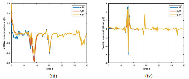
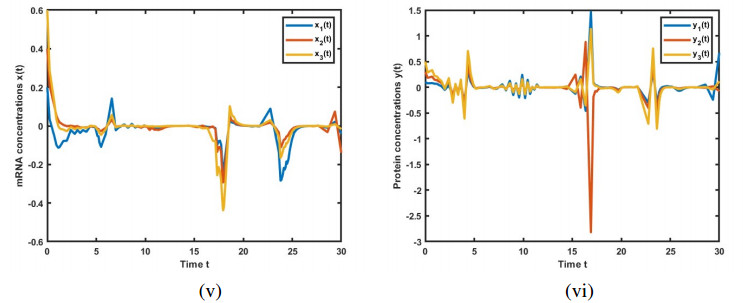
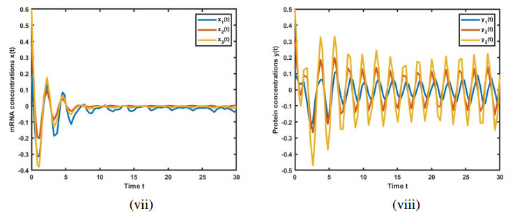
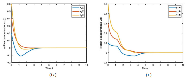
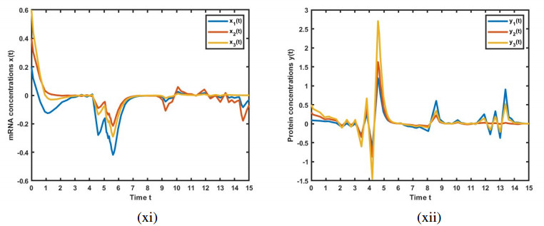
Figure 1 presents the solutions for GRN (3.14) in the absence of leakage delays. We observe that the solution for x(t) approaches 0 as t approaches 4, and the solution for y(t) approaches 0 as t approaches 5. In this case, the system converges to 0.
Figures 2–4 present the solutions for GRN (2.4), incorporating leakage delays. These figures clearly illustrate the interference caused by the system's leakage delays, impacting the convergence to the equilibrium point. We found that an increase in the leakage parameter has led to a corresponding rise in the frequency of the oscillations.
Figure 5 demonstrates the solutions of the GRNs (3.14) over the time interval t∈[0,10]. The solution for x(t) approaches 0 as t approaches 4, and the solution for y(t) approaches 0 as t approaches 5. In this case, the system converges to 0. While similar to Figure 1, the solution's behavior is observed over a shorter time interval in this instance.
Figure 6 shows the solutions of GRN (2.4) over the time interval t∈[0,15]. Notably, a disturbance in the solution is observed around t=3, where both x(t) and y(t) begin to oscillate. Despite this disturbance, the system remains stable. This scenario shows a similar solution trajectory to Figure 3 but over a shorter time span, which reduces the frequency of oscillations.
This comprehensive analysis of the simulation results provides valuable insights into the influence of leakage delays on the dynamics of GRNs (2.4) and (3.14). The analysis demonstrates the importance of considering such delays in the design and analysis of these systems. The leakage delay has a significant effect on the dynamic behaviors of the model, often leading to instability. It is therefore crucial to study stability while taking into account the impact of leakage delays.
Additionally, we examine the leakage delays effects by substituting the following values: In Case 1, we investigate the value of hM at rm=0.7,rM=1.2,rdm=−0.7,rdM=0.7,hm=1,hdm=−1,hdM=1, α=0.01,T=5, and varying leakage delays (ρa and ρc) as shown in Table 1. In Case 2, we will explore the value of rM at rm=0.7,rdm=−0.7,rdM=0.7,hm=1,hM=2,hdm=−1,hdM=1, α=0.01,T=5, and varying leakage delays as indicated in Table 2.
| ρa=ρc | 0.00 | 0.01 | 0.05 | 0.10 | 0.12 |
| Corollary 3.2 | 2.8741 | - | - | - | - |
| Theorem 3.1 | 2.8734 | 2.8067 | 2.5490 | 2.2491 | 2.1371 |
 DownLoad:
CSV
DownLoad:
CSV
| ρa=ρc | 0.00 | 0.01 | 0.05 | 0.10 | 0.12 |
| Corollary 3.2 | 6.6890 | - | - | - | - |
| Theorem 3.1 | 6.6890 | 6.6243 | 6.3692 | 6.0493 | 5.9209 |
DownLoad:
CSV
We observed that as the values of leakage delays ρa and ρc increases, the times delays hM and rM both decrease. Hence, it can be stated that the effects of leakage delays lead to a decrease in the FTS boundary.
In this paper, our focus is on investigating how leakage delays affect FTS in GRNs characterized by interval time-varying delays. To begin, we introduce GRNs that incorporate interval time-varying delays as well as leakage delays. These models consider lower bounds on delays, which may be either positive or zero, and allow for the derivatives of delays to be either positive or negative. Subsequently, we delve into the consequences of leakage delays through the construction of a LK function. We then enhance the criteria for FTS by employing estimates of integral inequalities and a reciprocally convex technique. This refinement enables us to express the new finite-time stability criteria for genetic regulatory networks in the form of LMIs. Finally, we present a numerical example to demonstrate the effect of leakage delays and validate the significance of our theoretical findings.
N.S. and I.K.: Conceptualization; N.S. and I.K.: Methodology; N.S. and I.K.: Software; N.S., K.M., and I.K.: Validation; I.K., N.S., and K.M.: Formal analysis; N.S., K.M., and I.K.: Investigation; N.S. and I.K.: Writing-original draft preparation; N.S., K.M., and I.K.: Writing-review and editing; N.S.and I.K.: Visualization; N.S., K.M., and I.K.: Supervision; N.S.: Project administration; N.S.: Funding acquisition. All authors have read and agreed to the published version of the manuscript.
The authors declare they have not used Artificial Intelligence (AI) tools in the creation of this article.
This work is supported by research and innovation funding from the Faculty of Agriculture and Technology, Nakhon Phanom University (Grant AG004/2566), and the Faculty of Engineering, Rajamangala University of Technology Isan Khon Kaen Campus.
The authors declare that there are no conflicts of interest regarding the publication of this manuscript
| [1] | Schäfer F, Lambert M, Christiansen E, et al. (2005) The Inter-agency space debris coordination committee (IADC) protection manual. Proceedings of the 4th European Conference on Space Debris, 39–44. |
| [2] |
Christiansen EL, Kerr JH (1993) Mesh double-bumper shield: a low-weight alternative for spacecraft meteoroid and orbital debris protection. Int J Impact Eng 14: 169–180. doi: 10.1016/0734-743X(93)90018-3

|
| [3] | Bezrukov LN, Gadasin IM, Kiselev AI, et al. (2000) About the physical bases of building the protection of the ISS module ―Zarya‖ against impact damage by near-earth space debris fragments. Cosmonautics Rocket Eng 18: 140–151 (in Russian). |
| [4] | Putzar R, Hupfer J, Aridon G, et al. (2013) Screening tests for enhanced shielding against hypervelocity particle impacts for future unmanned spacecraft. Proceedings of 6th European Conference on Space Debris. |
| [5] |
Horz F, Cintala MJ, Bernhard RP, et al. (1995) Multiple-mesh bumpers: a feasibility study. Int J Impact Eng 17: 431–442. doi: 10.1016/0734-743X(95)99868-R
|
| [6] | Semenov A, Bezrukov L, Malkin A, et al. (2006) Impact fragmentation dependence on geometrical parameter of single mesh bumpers. Mech Comp Mater Construct 12: 256–262. |
| [7] |
Higashide M, Tanaka M, Akahoshi Y, et al. (2006) Hypervelocity impact tests against metallic meshes. Int J Impact Eng 33: 335–342. doi: 10.1016/j.ijimpeng.2006.09.071
|
| [8] | Pang BJ, Lin M, Zhang K (2013) The Characteristics study of debris cloud of the mesh shields under hypervelocity impact. Proceedings of 6th European Conference on Space Debris. |
| [9] | Shumikhin TA, Myagkov NN, Bezrukov LN (2014) Distribution of kinetic energy among morphologically different parts of debris cloud at high velocity perforation of thin discrete bumpers by compact projectile. Mech Comp Mater Construct 20: 319–333 (in Russian). |
| [10] |
Myagkov NN, Shumikhin TA, Bezrukov LN (2010) Experimental and numerical study of peculiarities at high-velocity interaction between a projectile and discrete bumpers. Int J Impact Eng 37: 980–994. doi: 10.1016/j.ijimpeng.2010.04.001
|
| [11] | Sanchez GA, Christiansen EL (1996) FGB energy block meteoroid and orbital (M/OD) debris shield test report. JSC-27460, NASA Johnson Space Center, Houston. |
| [12] | Bezrukov LN, Shumikhin TA, Myagkov NN (2008) Ballistic properties of mesh shielding protection design under high-velocity impact. Mech Comp Mater Construct 14: 202–216 (in Russian). |
| [13] | Bezrukov LN, Gadasin IM, Shumikhin TA, et al. (2014) The testing of some prototypes of space debris shield protection. Mech Comp Mater Construct 20: 646–662 (in Russian). |
| [14] | Swift HF (1982) Hypervelocity impact mechanics, In: Zukas JA, Nicholas T, Swift HF, et al., Impact Dynamics, New York: John Wiley and Sons. |
| [15] | Hallquist JO (2007) LS-DYNA Keyword User's Manual, Version 971, Livermore Software Technology Corporation. |
| [16] |
Monaghan JJ (2005) Smoothed particle hydrodynamics. Rep Prog Phys 68: 1703–1759. doi: 10.1088/0034-4885/68/8/R01
|
| [17] |
Myagkov NN, Stepanov VV (2014) On projectile fragmentation at high-velocity perforation of a thin bumper. Physica A 410: 120–130. doi: 10.1016/j.physa.2014.05.021
|
| [18] | Zel'dovich YB, Raizer YP (1966) Physics of Shock Waves and High-Temperature Hydrodynamic Phenomena. New York: Academic. |
| [19] | Johnson GR (1983) A constitutive model and data for metals subjected to large strains, high strain rates and high temperatures. Proceedings of the 7th International Symposium on Ballistics, 541–547. |
| [20] | Kanel GI, Razorenov SV, Fortov VE, et al. (2004) Shock-Wave Phenomena and the Properties of Condensed Matter, New York: Springer-Verlag. |
| [21] |
Piekutowski AJ (1995) Fragmentation of a sphere initiated by hypervelocity impact with a thin sheet. Int J Impact Eng 17: 627–638. doi: 10.1016/0734-743X(95)99886-V
|
| 1. | Weike Duan, Jinsen Zhang, Liang Zhang, Zongsong Lin, Yuhang Chen, Xiaowei Hao, Yixin Wang, Hongri Zhang, Evaluation of an artificial intelligent hydrocephalus diagnosis model based on transfer learning, 2020, 99, 0025-7974, e21229, 10.1097/MD.0000000000021229 | |
| 2. | Peng Lu, Hao Xi, Bing Zhou, Hongpo Zhang, Yusong Lin, Liwei Chen, Yang Gao, Yabin Zhang, Yanhua Hu, Zhenghua Chen, A New Multichannel Parallel Network Framework for the Special Structure of Multilead ECG, 2020, 2020, 2040-2309, 1, 10.1155/2020/8889483 | |
| 3. | Babita Pandey, Devendra Kumar Pandey, Brijendra Pratap Mishra, Wasiur Rhmann, A comprehensive survey of deep learning in the field of medical imaging and medical natural language processing: Challenges and research directions, 2021, 13191578, 10.1016/j.jksuci.2021.01.007 | |
| 4. | Beanbonyka Rim, Nak-Jun Sung, Sedong Min, Min Hong, Deep Learning in Physiological Signal Data: A Survey, 2020, 20, 1424-8220, 969, 10.3390/s20040969 | |
| 5. | Sulaiman Somani, Adam J Russak, Felix Richter, Shan Zhao, Akhil Vaid, Fayzan Chaudhry, Jessica K De Freitas, Nidhi Naik, Riccardio Miotto, Girish N Nadkarni, Jagat Narula, Edgar Argulian, Benjamin S Glicksberg, Deep learning and the electrocardiogram: review of the current state-of-the-art, 2021, 1099-5129, 10.1093/europace/euaa377 | |
| 6. | Xu Wang, Runchuan Li, Shuhong Wang, Shengya Shen, Wenzhi Zhang, Bing Zhou, Zongmin Wang, Automatic diagnosis of ECG disease based on intelligent simulation modeling, 2021, 67, 17468094, 102528, 10.1016/j.bspc.2021.102528 | |
| 7. | Shuhong Wang, Runchuan Li, Xu Wang, Shengya Shen, Bing Zhou, Zongmin Wang, Chien Yu Chen, Multiscale Residual Network Based on Channel Spatial Attention Mechanism for Multilabel ECG Classification, 2021, 2021, 2040-2309, 1, 10.1155/2021/6630643 | |
| 8. | Nehemiah Musa, Abdulsalam Ya’u Gital, Nahla Aljojo, Haruna Chiroma, Kayode S. Adewole, Hammed A. Mojeed, Nasir Faruk, Abubakar Abdulkarim, Ifada Emmanuel, Yusuf Y. Folawiyo, James A. Ogunmodede, Abdukareem A. Oloyede, Lukman A. Olawoyin, Ismaeel A. Sikiru, Ibrahim Katb, A systematic review and Meta-data analysis on the applications of Deep Learning in Electrocardiogram, 2022, 1868-5137, 10.1007/s12652-022-03868-z | |
| 9. | Shan Wei Chen, Shir Li Wang, Xiu Zhi Qi, Suzani Mohamad Samuri, Can Yang, Review of ECG detection and classification based on deep learning: Coherent taxonomy, motivation, open challenges and recommendations, 2022, 74, 17468094, 103493, 10.1016/j.bspc.2022.103493 | |
| 10. | Ya'nan Wang, Sen Liu, Haijun Jia, Xintao Deng, Chunpu Li, Aiguo Wang, Cuiwei Yang, A two-step method for paroxysmal atrial fibrillation event detection based on machine learning, 2022, 19, 1551-0018, 9877, 10.3934/mbe.2022460 | |
| 11. | Qun Song, Tengyue Li, Simon Fong, Feng Wu, An ECG data sampling method for home-use IoT ECG monitor system optimization based on brick-up metaheuristic algorithm, 2021, 18, 1551-0018, 9076, 10.3934/mbe.2021447 | |
| 12. | Qinghua Sun, Zhanfei Xu, Chunmiao Liang, Fukai Zhang, Jiali Li, Rugang Liu, Tianrui Chen, Bing Ji, Yuguo Chen, Cong Wang, A dynamic learning-based ECG feature extraction method for myocardial infarction detection, 2022, 43, 0967-3334, 124005, 10.1088/1361-6579/acaa1a | |
| 13. | S. Immaculate Joy, K. Senthil Kumar, M. Palanivelan, D. Lakshmi, Review on Advent of Artificial Intelligence in Electrocardiogram for the Detection of Extra-Cardiac and Cardiovascular Disease, 2023, 46, 2694-1783, 99, 10.1109/ICJECE.2022.3228588 | |
| 14. | Enes Efe, Emrehan Yavsan, AttBiLFNet: A novel hybrid network for accurate and efficient arrhythmia detection in imbalanced ECG signals, 2024, 21, 1551-0018, 5863, 10.3934/mbe.2024259 |
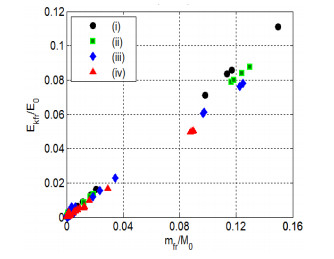
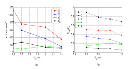
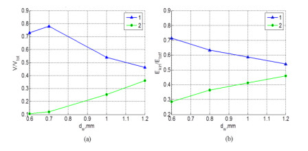
Nikolay Myagkov, Timofey Shumikhin. Studying the redistribution of kinetic energy between the morphologically distinct parts of the fragments cloud formed from high-velocity impact fragmentation of an aluminum sphere on a steel mesh[J]. AIMS Materials Science, 2019, 6(5): 685-696. doi: 10.3934/matersci.2019.5.685

| ρa=ρc | 0.00 | 0.01 | 0.05 | 0.10 | 0.12 |
| Corollary 3.2 | 2.8741 | - | - | - | - |
| Theorem 3.1 | 2.8734 | 2.8067 | 2.5490 | 2.2491 | 2.1371 |
DownLoad:
CSV
| ρa=ρc | 0.00 | 0.01 | 0.05 | 0.10 | 0.12 |
| Corollary 3.2 | 6.6890 | - | - | - | - |
| Theorem 3.1 | 6.6890 | 6.6243 | 6.3692 | 6.0493 | 5.9209 |
DownLoad:
CSV