Recent coating materials for textile-based solar cells

Andrea Ehrmann; Tomasz Blachowicz; Andrea Ehrmann; Tomasz Blachowicz

doi:10.3934/matersci.2019.2.234

AIMS Materials Science

2019, Volume 6, Issue 2: 234-251. doi: 10.3934/matersci.2019.2.234

Previous Article Next Article

Mini review Special Issues

Recent coating materials for textile-based solar cells

Andrea Ehrmann ^{1
,
,},
Tomasz Blachowicz ²

1.
ITES, Faculty of Engineering and Mathematics, Bielefeld University of Applied Sciences, 33619 Bielefeld, Germany
2.
Institute of Physics – Center of Science and Education, Silesian University of Technology, 44-100 Gliwice, Poland

Received: 29 December 2018 Accepted: 19 March 2019 Published: 28 March 2019

Electronic textiles may be used to monitor a person’s vital function, to offer information or navigation, and to support people in daily life. One crucial problem, however, is the energy supply needed for such electronic functions. One of the possibilities discussed for this purpose is the integration of solar cells into garments. While silicon-based solar cells are mostly rigid or can in the meantime also be prepared in the shape of relatively flexible foils, the approach to integrate solar cell functionality into a textile fabric goes one step further. In this case, dye-sensitized solar cells (DSSCs), polymer or organic solar cells are advantageous. During the last years, promising advances are reported in the literature, discussing new materials for the different layers of such flexible solar cells. This review gives an overview of the recent materials used for creating flexible solar cells on textile fabrics or fibers.
- dye-sensitized solar cells,
- DSSC,
- polymer solar cell,
- organic solar cell,
- inorganic,
- electrodes,
- cathode,
- anode,
- electrolyte
Citation: Andrea Ehrmann, Tomasz Blachowicz. Recent coating materials for textile-based solar cells[J]. AIMS Materials Science, 2019, 6(2): 234-251. doi: 10.3934/matersci.2019.2.234

Related Papers:

Abstract

Electronic textiles may be used to monitor a person’s vital function, to offer information or navigation, and to support people in daily life. One crucial problem, however, is the energy supply needed for such electronic functions. One of the possibilities discussed for this purpose is the integration of solar cells into garments. While silicon-based solar cells are mostly rigid or can in the meantime also be prepared in the shape of relatively flexible foils, the approach to integrate solar cell functionality into a textile fabric goes one step further. In this case, dye-sensitized solar cells (DSSCs), polymer or organic solar cells are advantageous. During the last years, promising advances are reported in the literature, discussing new materials for the different layers of such flexible solar cells. This review gives an overview of the recent materials used for creating flexible solar cells on textile fabrics or fibers.

References

[1]	Schubert MB, Werner JH (2006) Flexible solar cells for clothing. Mater Today 9: 42–50.
[2]	Kim W, Kwon S, Lee SM, et al. (2013) Soft fabric-based flexible organic light-emitting diodes. Org Electron 14: 3007–3013. doi: 10.1016/j.orgel.2013.09.001
[3]	Jung JW, Williams ST, Jen AKY (2014) Low-temperature processed high-performance flexible perovskite solar cells via rationally optimized solvent washing treatments. RSC Adv 4: 62971–62977. doi: 10.1039/C4RA13212B
[4]	Jeong I, Kim HJ, Lee BS, et al. (2015) Highly efficient perovskite solar cells based on mechanically durable molybdenum cathode. Nano Energy 17: 131–139. doi: 10.1016/j.nanoen.2015.07.025
[5]	O'Regan B, Grätzel M (1991) A low-cost, high-efficiency solar cell based on dye-sensitized colloidal TiO₂ films. Nature 353: 737–740. doi: 10.1038/353737a0
[6]	Ye M, Wen X, Wang M, et al. (2015) Recent advances in dye-sensitized solar cells: from photoanodes, sensitizers and electrolytes to counter electrodes. Mater Today 18: 155–162. doi: 10.1016/j.mattod.2014.09.001
[7]	Pan J, Smritakshi P, Murali B, et al. (2015) Air-stable surface-passivated perovskite quantum dots for ultra-robust, single- and two-photon-induced amplified spontaneous emission. J Phys Chem 6: 5027–5033.
[8]	Yang YM, Chen W, Dou L, et al. (2015) High-performance multiple-donor bulk heterojunction solar cells. Nat Photonics 9: 190–198. doi: 10.1038/nphoton.2015.9
[9]	Li Y, Xu G, Cui C, et al. (2018) Flexible and semitransparent organic solar cells. Adv Energy Mater 8: 1701791. doi: 10.1002/aenm.201701791
[10]	Yang W, Park B, Jung E, et al. (2017) Iodide management in formamidinium-lead-halide-based perovskite layers for efficient solar cells. Science 356: 1376–1379. doi: 10.1126/science.aan2301
[11]	Zhang H, Cheng J, Lin F, et al. (2016) Pinhole-free and surface-nanostructured NiO_X film by room-temperature solution process for high-performance flexible perovskite solar cells with good stability and reproducibility. ACS Nano 10: 1503–1511. doi: 10.1021/acsnano.5b07043
[12]	Roldán-Carmona C, Malinkiewicz O, Soriano A, et al. (2014) Flexible high efficiency perovskite solar cells. Energ Environ Sci 7: 994–997. doi: 10.1039/c3ee43619e
[13]	Wang D, Wright M, Elumalai NK, et al. (2016) Stability of perovskite solar cells. Sol Energ Mat Sol C 147: 255–275. doi: 10.1016/j.solmat.2015.12.025
[14]	Ji XY, Cheng HY, Grede AJ, et al. (2018) Conformal coating of amorphous silicon and germanium by high pressure chemical vapor deposition for photovoltaic fabrics. APL Mater 6: 046105. doi: 10.1063/1.5020814
[15]	Ehrmann A, Blachowicz T (2019) Comment on 'Dye-sensitized solar cells using Aloe Vera and Cladode of Cactus extracts as natural sensitizers' [Chem. Phys. Lett. 679 (2017) 97–101]. Chem Phys Lett 714: 227–229.
[16]	Plentz J, Andra G, Pliewischkies T, et al. (2016) Amorphous silicon thin-film solar cells on glass fiber textiles. Mater Sci Eng B-Adv 204: 34–37. doi: 10.1016/j.mseb.2015.11.007
[17]	Liu JQ, Li Y, Yong S, et al. (2019) Flexible printed monolithic-structured solid-state dye sensitized solar cells on woven glass fibre textiles for wearable energy harvesting applications. Sci Rep 9: 1362. doi: 10.1038/s41598-018-37590-8
[18]	Li Y, Arumugam S, Krishnan C, et al. (2019) Encapsulated textile organic solar cells fabricated by spray coating. Chemistry Select 4: 407–412.
[19]	Liang X, Long GH, Fu CW, et al. (2018) High performance all-solid-state flexible supercapacitor for wearable storage device application. Chem Eng J 345: 186–195.
[20]	Ji XY, Cheng HY, Grede AJ, et al. (2018) Conformal coating of amorphous silicon and germanium by high pressure chemical vapor deposition for photovoltaic fabrics. APL Mater 6: 046105. doi: 10.1063/1.5020814
[21]	Grancaric AM, Jerkovic I, Koncar V, et al. (2018) Conductive polymers for smart textile applications. J Ind Text 48: 612–642. doi: 10.1177/1528083717699368
[22]	Kye MJ, Cho JH, Yu JC, et al. (2018) "Drop-on-textile" patternable aqueous PEDOT composite ink providing highly stretchable and wash-resistant electrodes for electronic textiles. Dyes Pigments 155: 150–158. doi: 10.1016/j.dyepig.2018.03.024
[23]	Fu XM, Xu LM, Li JX, et al. (2018) Flexible solar cells based on carbon nanomaterials. Carbon 139: 1063–1073. doi: 10.1016/j.carbon.2018.08.017
[24]	Li LB, Zhang S, Yang ZC, et al. (2018) Recent advances of flexible perovskite solar cells. J Energy Chem 27: 673–689.
[25]	Tsuboi K, Matsumoto H, Fukawa T, et al. (2015) Simulation study on optical absorption property of fiber- and fabric-shaped organic thin-film solar cells with resin sealing layer. Sen-I Gakkaishi 71: 121–126. doi: 10.2115/fiber.71.121
[26]	Peng M, Dong B, Zou C (2018) Three dimensional photovoltaic fibers for wearable energy harvesting and conversion. J Energy Chem 27: 611–621. doi: 10.1016/j.jechem.2018.01.008
[27]	Koops SE, O'Regan BC, Barnes PRF, et al. (2009) Parameters influencing the efficiency of electron injection in dye-sensitized solar cells. J Am Chem Soc 131: 4808–4818. doi: 10.1021/ja8091278
[28]	Sabet M, Salavati-Niasari M (2014) Deposition of cadmium selenide semiconductor nanostructures on TiO₂ surface via different chemical methods and investigation of their effects on dye sensitized solar cell efficiency. Mat Sci Semicon Proc 27: 619–633. doi: 10.1016/j.mssp.2014.07.031
[29]	Lei Y, Yang C, Hou J, et al. (2017) Strongly coupled CdS/graphene quantum dots nanohybrids for highly efficient photocatalytic hydrogen evolution: Unraveling the essential roles of graphene quantum dots. Appl Catal B-Environ 216: 59–69. doi: 10.1016/j.apcatb.2017.05.063
[30]	Kundu S, Sarojinijeeva P, Karthick R, et al. (2017) Enhancing the efficiency of DSSCs by the modification of TiO₂ photoanodes using N, F and S, co-doped graphene quantum dots. Electromchim Acta 242: 337–343.
[31]	Grissom G, Jaksik J, McEntee M, et al. (2018) Three-dimensional carbon nanotube yarn based solid state solar cells with multiple sensitizers exhibit high energy conversion efficiency. Sol Energy 171: 16–22. doi: 10.1016/j.solener.2018.06.053
[32]	Sánchez-García MA, Bokhimi X, Velázquez Martinez S, et al. (2018) Dye-Sensitized Solar Cells Prepared with Mexican Pre-Hispanic Dyes. J Nanotechnol 2018: 1236878.
[33]	Juhász Junger I, Grimmelsmann N, Homburg SV, et al. (2017) Einfluss des pH-Wertes von Anthocyan-Farbstoffen auf die elektrischen Eigenschaften von Farbstoffsolarzellen. Proceedings des Fachgruppentreffen des Graduierteninstituts NRW-Ressourcen, Bochum, Germany.
[34]	Zhang X, Zhang J, Liu J, et al. (2015) Solution processed flexible and bending durable heterojunction colloidal quantum dot solar cell. Nanoscale 7: 11520–11524. doi: 10.1039/C5NR02617B
[35]	Zhang X, Johansson EMJ (2016) Utilizing light trapping interference effects in microcavity structured colloidal quantum dot solar cells: A combined theoretical and experimental approach. Nano Energy 28: 71–77. doi: 10.1016/j.nanoen.2016.08.034
[36]	Zhang X, Aitola K, Hagglund C, et al. (2017) Dry-deposited transparent carbon nanotube film as front electrode in colloidal quantum dot solar cells. ChemSusChem 10: 434–441. doi: 10.1002/cssc.201601254
[37]	Liu M, Voznyy O, Sabatini R, et al. (2017) Hybrid organic–inorganic inks flatten the energy landscape in colloidal quantum dot solids. Nat Mater 16: 258–263. doi: 10.1038/nmat4800
[38]	Zhang XL, Öberg VA, Du J, et al. (2018) Extremely lightweight and ultra-flexible infrared light-converting quantum dot solar cells with high power-per-weight output using a solution-processed bending durable silver nanowire-based electrode. Energ Environ Sci 11: 354. doi: 10.1039/C7EE02772A
[39]	Liu J, Li Y, Arumugam S, et al. (2018) Screen printed dye-sensitized solar cells (DSSCs) on Woven polyester cotton fabric for wearable energy harvesting applications. Mater Today Proc 5: 13753–13758.
[40]	Liu J, Li Y, Arumugam S, et al. (2018) Investigation of low temperature processed titanium dioxide (TiO₂) films for printed dye sensitized solar cells (DSSCs) for large area flexible applications. Mater Today Proc 5: 13846–13854.
[41]	Juhász Junger I, Homburg SV, Grethe T, et al. (2017) Examination of the sintering process-dependent properties of TiO₂ on glass and textile substrates. J Photon Energy 7: 015001. doi: 10.1117/1.JPE.7.015001
[42]	Herrmann A, Fiedler J, Ehrmann A, et al. (2016) Examination of the sintering process dependent micro- and nanostructure of TiO₂ on textile substrates. Photonics for Solar Energy Systems VI. International Society for Optics and Photonics, 9898: 98980S doi: 10.1117/12.2227180
[43]	Opwis K, Gutmann JS, Lagunas Alonso AR, et al. (2016) Preparation of a textile-based dye-sensitized solar cell. Int J Photoenergy 2016: 3796074.
[44]	Jun MJ, Cha SI, Seo SH, et al. (2016) Float printing deposition to control the morphology of TiO₂ photoanodes on woven textile metal substrates for TCO-free flexible dye-sensitized solar cells. RSC Adv 6: 67331–67339. doi: 10.1039/C6RA09457K
[45]	Krämer A, Engel S, Sangiorgi N, et al. (2017) ZnO thin films on single carbon fibres fabricated by Pulsed Laser Deposition (PLD). Appl Surf Sci 399: 282–287. doi: 10.1016/j.apsusc.2016.12.046
[46]	Rezaei B, Soleimany R, Ensafi AA, et al. (2018) Photocatalytic degradation enhancements of dyes with bi-functionalized zones of modified nanoflower like TiO₂ with Pt-C₃N₄ under sunlight irradiation. J Environ Chem Eng 6: 7010–7020.
[47]	Das PP, Roy A, Tathavadekar M, et al. (2017) Photovoltaic and photocatalytic performance of electrospun Zn₂SnO₄ hollow fibers. Appl Catal B-Environ 203: 692–703. doi: 10.1016/j.apcatb.2016.10.035
[48]	Fan X, Chu ZZ, Wang FZ, et al. (2008) Wire-shaped flexible dye-sensitized solar cells. Adv Mater 20: 592. doi: 10.1002/adma.200701249
[49]	Pu X, Song WX, Liu MM, et al. (2016) Wearable power-textiles by integrating fabric triboelectric nanogenerators and fiber-shaped dye-sensitized solar cells. Adv Energy Mater 6: 1601048. doi: 10.1002/aenm.201601048
[50]	Wen Z, Yeh MH, Guo H, et al. (2016) Self-powered textile for wearable electronics by hybridizing fiber-shaped nanogenerators, solar cells, and supercapacitors. Sci Adv 2: e1600097. doi: 10.1126/sciadv.1600097
[51]	Yang Z (2016) High performance fiber-shaped solar cells. Pure Appl Chem 88: 113–117.
[52]	Yun MJ, Cha SI, Kim HS, et al. (2016) Monolithic-structured single-layered textile-based dye-sensitized solar cells. Sci Rep 6: 34249. doi: 10.1038/srep34249
[53]	Chai ZS, Zhang NN, Sun P, et al. (2016) Tailorable and wearable textile devices for solar energy harvesting and simultaneous storage. ACS Nano 10: 9201–9207. doi: 10.1021/acsnano.6b05293
[54]	Chen J, Huang Y, Zhang NN, et al. (2016) Micro-cable structured textile for simultaneously harvesting solar and mechanical energy. Nat Energy 1: 16138. doi: 10.1038/nenergy.2016.138
[55]	Weintraub B, Wei Y, Wang ZL (2009) Optical fiber/nanowire hybrid structures for efficient three-dimensional dye-sensitized solar cells. Angew Chem 48: 8981. doi: 10.1002/anie.200904492
[56]	Juhász Junger I, Großerhode C, Storck JL, et al. (2018) Influence of graphite-coating methods on the DSSC performance. Optik 174: 40–45. doi: 10.1016/j.ijleo.2018.08.041
[57]	Grötsch G, Cornelißen C, Streitenberger A, et al. (2018) Development of textile-based organic photovoltaics. Proceedings of Aachen-Dresden-Denkendorf International Textile Conference.
[58]	Mengal N, Arbab AA, Sahito IA, et al. (2017) An electrocatalytic active lyocell fabric cathode based on cationically functionalized and charcoal decorated graphite composite for quasi-solid state dye sensitized solar cell. Sol Energy 155: 110–120. doi: 10.1016/j.solener.2017.06.032
[59]	Memon AA, Arbab AA, Iftikhar A, et al. (2017) Synthesis of highly photo-catalytic and electro-catalytic active textile structured carbon electrode and its application in DSSCs. Sol Energy 150: 521–531. doi: 10.1016/j.solener.2017.04.052
[60]	Sahito IA, Sun KC, Arbab AA, et al. (2016) Flexible and conductive cotton fabric counter electrode coated with graphene nanosheets for high efficiency dye sensitized solar cell. J Power Sources 319: 90–98.
[61]	Arbab AA, Sun KC, Sahito IA, et al. (2016) Fabrication of textile fabric counter electrodes using activated charcoal doped multi walled carbon nanotube hybrids for dye sensitized solar cells. J Mater Chem A 4: 1495–1505. doi: 10.1039/C5TA08858E
[62]	Motlagh MS, Mottaghitalab V (2017) The charge transport characterization of the polyaniline coated carbon fabric as a novel textile based counter electrode for flexible dye-sensitized solar cell. Electrochim Acta 249: 308–317.
[63]	Juhász L, Juhász Junger I (2018) Spectral analysis and parameter identification of textile-based dye-sensitized solar cells. Materials 11: 1623. doi: 10.3390/ma11091623
[64]	Juhász Junger I, Wehlage D, Böttjer R, et al. (2018) Dye-sensitized solar cells with electrospun nanofiber mat-based counter electrodes. Materials 11: 1604. doi: 10.3390/ma11091604
[65]	Xu Q, Li M, Yan P, et al. (2016) Polypyrrole-coated cotton fabrics prepared by electrochemical polymerization as textile counter electrode for dye-sensitized solar cells. Org Electron 29: 107–113.
[66]	Juhász Junger I, Tellioglu A, Ehrmann A (2018) Refilling DSSCs as a method to ensure longevity. Optik 160: 255–258. doi: 10.1016/j.ijleo.2018.01.123
[67]	Sahito IA, Ahmed F, Khatri Z, et al. (2017) Enhanced ionic mobility and increased efficiency of dye-sensitized solar cell by adding lithium chloride in poly(vinylidene fluoride) nanofiber as electrolyte medium. J Mater Sci 52: 13920–13929. doi: 10.1007/s10853-017-1473-z
[68]	Sun KC, Sahito IA, Noh JW, et al. (2016) Highly efficient and durable dye-sensitized solar cells based on a wet-laid PET membrane electrolyte. J Mater Chem A 4: 458–465. doi: 10.1039/C5TA07720F
[69]	Hölscher F, Trümper PR, Juhász Junger I, et al. (2018) Raising reproducibility in dye-sensitized solar cells under laboratory conditions. J Renew Sustain Ener 10: 013506. doi: 10.1063/1.5013181
[70]	Bedeloglu A, Demir A, Bozkurt Y, et al. (2009) A flexible textile structure based on polymeric photovoltaics using transparent cathode. Synthetic Met 159: 2043–2048. doi: 10.1016/j.synthmet.2009.07.019
[71]	Bedeloglu A, Koeppe R, Demir A, et al. (2010) Development of energy generating photovoltaic textile structures for smart applications. Fiber Polym 11: 378–383. doi: 10.1007/s12221-010-0378-0
[72]	Bedeloglu A, Demir A, Bozkurt Y, et al. (2010) Photovoltaic properties of polymer based organic solar cells adapted for non-transparent substrates. Renew Energ 35: 2301–2306. doi: 10.1016/j.renene.2010.02.030
[73]	Bedeloglu A, Jimenez P, Demir A, et al. (2011) Photovoltaic textile structure using polyaniline/carbon nanotube composite materials. J Text I 102: 857–862. doi: 10.1080/00405000.2010.525816
[74]	Krebs FC, Biancardo M, Winther-Jensen B, et al. (2006) Strategies for incorporation of polymer photovoltaics into garments and textiles. Sol Energ Mat Sol C 90: 1058–1067. doi: 10.1016/j.solmat.2005.06.003
[75]	Arumugam S, Li Y, Liu J, et al. (2018) Optimized process of fully spray-coated organic solar cells on woven polyester cotton fabrics. Mater Today Proc 5: 13745–13752.
[76]	Arumugam S, Li Y, Senthilarasu S, et al. (2016) Fully spray-coated organic solar cells on woven polyester cotton fabrics for wearable energy harvesting applications. J Mater Chem A 4: 5561–5568. doi: 10.1039/C5TA03389F
[77]	Zhen HY, Li K, Chen CJ, et al. (2017) Water-borne foldable polymer solar cells: one-step transferring free-standing polymer films onto woven fabric electrodes. J Mater Chem A 5: 782–788. doi: 10.1039/C6TA08309A
[78]	O'Connor B, Pipe KP, Shtein M (2008) Fiber based organic photovoltaic devices. Appl Phys Lett 92: 193306. doi: 10.1063/1.2927533
[79]	Bedeloglu A, Demir A, Bozkurt Y, et al. (2010) A photovoltaic fiber design for smart textiles. Text Res J 80: 1065–1074. doi: 10.1177/0040517509352520
[80]	Zou D, Lv Z, Cai X, et al. (2012) Macro/microfiber-shaped electronic devices. Nano Energy 1: 273–281. doi: 10.1016/j.nanoen.2012.01.005
[81]	Sugino K, Ikeda Y, Yonezawa S, et al. (2017) Development of fiber and textile-shaped organic solar cells for smart textiles. J Fiber Sci Technol 73: 336–342. doi: 10.2115/fiberst.2017-0049
[82]	Ebner M, Schennach R, Chien HT, et al. (2017) Regenerated cellulose fiber solar cell. Flex Print Electron 2: 014002. doi: 10.1088/2058-8585/aa5707
[83]	Wu CX, Kim TW, Guo TL, et al. (2017) Wearable ultra-lightweight solar textiles based on transparent electronic fabrics. Nano Energy 32: 367–373. doi: 10.1016/j.nanoen.2016.12.040
[84]	Liu P, Gao Z, Xu LM, et al. (2018) Polymer solar cell textiles with interlaced cathode and anode fibers. J Mater Chem A 6: 19947–19953. doi: 10.1039/C8TA06510A
[85]	Jinno H, Fukuda K, Xu XM, et al. (2017) Stretchable and waterproof elastomer-coated organic photovoltaics for washable electronic textile applications. Nat Energy 2: 780–785. doi: 10.1038/s41560-017-0001-3
[86]	Jung JW, Bae JH, Ko JH, et al. (2018) Fully solution-processed indium tin oxide-free textile-based flexible solar cells made of an organic–inorganic perovskite absorber: Toward a wearable power source. J Power Sources 402: 327–332. doi: 10.1016/j.jpowsour.2018.09.038
[87]	Ma MM, Tang QW, Chen HY, et al. (2017) Filling perovskite (5-AVA)_y(CH₃NH₃)_1−yPbI₃ or (5-AVA)_y(CH₃NH₃)_1−yPbI_3−xCl_x halide in a 3D gel framework for multideformable perovskite solar cell. Sol Energ Mat Sol C 160: 67–76. doi: 10.1016/j.solmat.2016.09.047
[88]	Lam JY, Chen JY, Tsai PC, et al. (2017) A stable, efficient textile-based flexible perovskite solar cell with improved washable and deployable capabilities for wearable device applications. RSC Adv 7: 54361–54368.
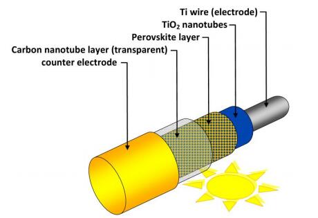
[89]	Wang XY, Kulkarni SA, Li Z, et al. (2016) Wire-shaped perovskite solar cell based on TiO₂ nanotubes. Nanotechnology 27: 20LT01.
[90]	Li HJ, Li XD, Wang WY, et al. (2019) Highly foldable and efficient paper-based perovskite solar cells. RRL Solar 3: 1800317. doi: 10.1002/solr.201800317
[91]	Castro-Hermosa S, Dagar J, Marsella A, et al. (2017) Perovskite solar cells on paper and the role of substrates and electrodes on performance. IEEE Electr Device L 38: 1278–1281. doi: 10.1109/LED.2017.2735178

Reader Comments

Your name:*

Email:*
© 2019 the Author(s), licensee AIMS Press. This is an open access article distributed under the terms of the Creative Commons Attribution License (http://creativecommons.org/licenses/by/4.0)