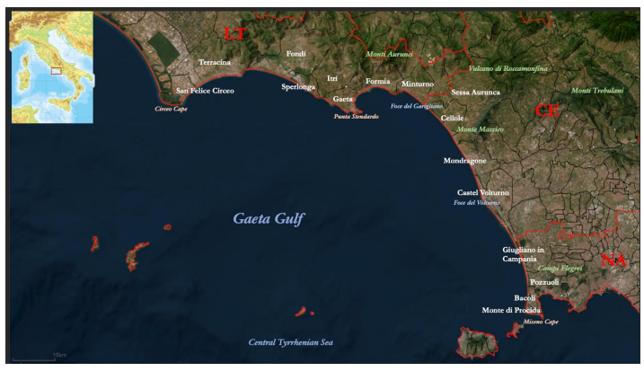
The coasts, with their intricate combination of natural and anthropogenic fragilities, can always be considered a crucial component in the geography of risk and territorial governance. Furthermore, coastal areas worldwide are currently facing profound and immediate impacts of climate change, presenting unparalleled challenges for both ecosystems and coastal communities. In these contexts, high socio-environmental vulnerability has often been linked to planning and management practices that, at times, have exacerbated coastal exposure, making it more prone to extreme natural phenomena, such as coastal floods and storm surges, as well as degradation. The case of the Gaeta Gulf, a largely urbanized part of the central Tyrrhenian coast in Italy that encompasses two administrative areas between the northern Campania and the southern Lazio Regions, provides an opportunity to investigate these criticalities both along the coastline and within the interconnected inland areas. This research aims to understand how administrations and communities perceive, experience, and understand the coastal risks and challenges posed by climate change, as well as their level of information and preparedness to address such risks. These aspects will be analyzed through a multidisciplinary approach, shedding light on the political, social, environmental, and economic practices in these areas, and the potential implications for coastal planning policies. In addition, this contribution presents the results of a qualitative survey involving the administration of questionnaires related to the perception of climate change impacts on the coasts and the level of information on the mitigation and adaptation practices within the communities living in these areas.
Citation: Eleonora Gioia, Eleonora Guadagno. Perception of climate change impacts, urbanization, and coastal planning in the Gaeta Gulf (central Tyrrhenian Sea): A multidimensional approach[J]. AIMS Geosciences, 2024, 10(1): 80-106. doi: 10.3934/geosci.2024006
The coasts, with their intricate combination of natural and anthropogenic fragilities, can always be considered a crucial component in the geography of risk and territorial governance. Furthermore, coastal areas worldwide are currently facing profound and immediate impacts of climate change, presenting unparalleled challenges for both ecosystems and coastal communities. In these contexts, high socio-environmental vulnerability has often been linked to planning and management practices that, at times, have exacerbated coastal exposure, making it more prone to extreme natural phenomena, such as coastal floods and storm surges, as well as degradation. The case of the Gaeta Gulf, a largely urbanized part of the central Tyrrhenian coast in Italy that encompasses two administrative areas between the northern Campania and the southern Lazio Regions, provides an opportunity to investigate these criticalities both along the coastline and within the interconnected inland areas. This research aims to understand how administrations and communities perceive, experience, and understand the coastal risks and challenges posed by climate change, as well as their level of information and preparedness to address such risks. These aspects will be analyzed through a multidisciplinary approach, shedding light on the political, social, environmental, and economic practices in these areas, and the potential implications for coastal planning policies. In addition, this contribution presents the results of a qualitative survey involving the administration of questionnaires related to the perception of climate change impacts on the coasts and the level of information on the mitigation and adaptation practices within the communities living in these areas.

| [1] | Lee H, Calvin K, Dasgupta D, et al. (2023) Climate Change 2023: Synthesis Report. Contribution of Working Groups Ⅰ, Ⅱ and Ⅲ to the Sixth Assessment Report of the Intergovernmental Panel on Climate Change. Geneva: IPCC. https://doi.org/10.59327/IPCC/AR6-9789291691647 |
| [2] |
Mentaschi L, Vousdoukas MI, Pekel J, et al. (2018) Global long-term observations of coastal erosion and accretion. Sci Rep 8: 1–11. https://doi.org/10.1038/s41598-018-30904-w doi: 10.1038/s41598-018-30904-w

|
| [3] |
Ribot JC (2011) Vulnerability before adaptation: Toward transformative climate action. Glob Environ Chang 21: 1160–1162. https://doi.org/10.1016/j.gloenvcha.2011.07.008 doi: 10.1016/j.gloenvcha.2011.07.008
|
| [4] | Casareale C, Gioia E, Colocci A, et al. (2023) Perception of the Self–Exposure to Geohazards in the Italian Coastal Population of the Adriatic Basin. In: D'Amico S, De Pascale F (Eds), Geohazards and Disaster Risk Reduction. Advances in Natural and Technological Hazards Research, London: Springer International Publishing, 49–71. https://doi.org/10.1007/978-3-031-24541-1_3 |
| [5] |
Sundblad EL, Biel A, Gä rling T (2007) Cognitive and affective risk judgements related to climate change. J Environ Psychol 27: 97–106. https://doi.org/10.1016/j.jenvp.2007.01.003 doi: 10.1016/j.jenvp.2007.01.003
|
| [6] |
Cutter SL, Barnes L, Berry M, et al. (2008) A place-based model for understanding community resilience to natural disasters. Glob Environ Chang 18: 598–606. https://doi.org/10.1016/j.gloenvcha.2008.07.013 doi: 10.1016/j.gloenvcha.2008.07.013
|
| [7] |
Gierlach E, Belsher BE, Beutler LE (2010) Cross-Cultural Differences in Risk Perceptions of Disasters. Risk Anal 30: 1539–1549. https://doi.org/10.1111/j.1539-6924.2010.01451.x doi: 10.1111/j.1539-6924.2010.01451.x
|
| [8] |
Reynolds TW, Bostrom A, Read D, et al. (2010) Now What Do People Know About Global Climate Change? Survey Studies of Educated Laypeople. Risk Anal 30: 1520–1538. https://doi.org/10.1111/j.1539-6924.2010.01448.x doi: 10.1111/j.1539-6924.2010.01448.x
|
| [9] |
Slovic P (1987) Perception of risk. Science 236: 280–285. https://doi.org/10.1126/science.3563507 doi: 10.1126/science.3563507
|
| [10] |
Bubeck P, Botzen WJW, Aerts JCJH (2012) A Review of Risk Perceptions and Other Factors that Influence Flood Mitigation Behavior. Risk Anal 32: 1481–1495. https://doi.org/10.1111/j.1539-6924.2011.01783.x doi: 10.1111/j.1539-6924.2011.01783.x
|
| [11] |
Wachinger G, Renn O, Begg C, et al. (2013) The risk perception paradox—implications for governance and communication of natural hazards. Risk Anal 33: 1049–1065. https://doi.org/10.1111/j.1539-6924.2012.01942.x doi: 10.1111/j.1539-6924.2012.01942.x
|
| [12] |
Grothmann T, Patt A (2005) Adaptive capacity and human cognition: The process of individual adaptation to climate change. Glob Environ Chang 15: 199–213. https://doi.org/10.1016/j.gloenvcha.2005.01.002 doi: 10.1016/j.gloenvcha.2005.01.002
|
| [13] |
Ernoul L, Vareltzidou S, Charpentier M, et al. (2020) Perception of climate change and mitigation strategies in two European Mediterranean deltas. AIMS Geosci 6: 561–576. https://doi.org/10.3934/geosci.2020032 doi: 10.3934/geosci.2020032
|
| [14] |
Lugeri FR, Farabollini P, De Pascale F, et al. (2021) PPGIS applied to environmental communication and hazards for a community—based approach: a dualism in the Southern Italy "calanchi" landscape. AIMS Geosci 7: 490–506. https://doi.org/10.3934/geosci.2021028 doi: 10.3934/geosci.2021028
|
| [15] |
Gugg G (2019) Beyond the volcanic risk. To defuse the announced disaster of Vesuvius. AIMS Geosci 5: 480–492. https://doi.org/10.3934/geosci.2019.3.480 doi: 10.3934/geosci.2019.3.480
|
| [16] | Ministry for the Environment Land and Sea (2007) Fourth National Communication under the UN Framework Convention on Climate Change. Rome: MATTM. |
| [17] | Lionello P, Baldi M, Brunetti M, et al. (2009) Eventi climatici estremi: tendenze attuali e clima futuro dell'Italia. In: Castellari S, Artale V (Eds), I cambiamenti climatici in Italia: evidenze, vulnerabilità e impatti, Bologna: Bononia University Press, 81–106. |
| [18] | Breil M, Catenacci M, Travisi C (2007) Impatti del cambiamento climatico sulle zone costiere: Quantificazione economica di impatti e di misure di adattamento—sintesi di risultati e indicazioni metodologiche per la ricerca futura. Conference paper prepared for the APAT Workshop on "Cambiamenti climatici e ambiente marino–costiero: scenari futuri per un programma nazionale di adattamento", Palermo. 27–28. |
| [19] | Woodroffe CD (2007) The natural resilience of coastal system: primary concepts, Managing Coastal Vulnerability, Amsterdam: Elsevier, 45–60. |
| [20] |
Salvati P, Bianchi C, Fiorucci F, et al. (2014) Perception of flood and landslide risk in Italy: A preliminary analysis. Nat Hazards Earth Syst Sci 14: 2589–2603. https://doi.org/10.5194/nhess-14-2589-2014 doi: 10.5194/nhess-14-2589-2014
|
| [21] |
Gioia E, Casareale C, Colocci A, et al. (2021) Citizens' Perception of Geohazards in Veneto Region (NE Italy) in the Context of Climate Change. Geosciences 11: 424. https://doi.org/10.3390/geosciences11100424 doi: 10.3390/geosciences11100424
|
| [22] |
Antronico L, Coscarelli R, Gariano SL, et al. (2023) Perception of climate change and geo-hydrological risk among high-school students: A local-scale study in Italy. Int J Disaster Risk Reduct 90: 103663. https://doi.org/10.1016/j.ijdrr.2023.103663 doi: 10.1016/j.ijdrr.2023.103663
|
| [23] |
Mercatanti L, Sabato G (2021) Sustainability and risk perception: multidisciplinary approaches, AIMS Geosci 7: 219–223. https://doi.org/10.3934/geosci.2021013 doi: 10.3934/geosci.2021013
|
| [24] |
Bonati S (2021) Dal climate denial alla natura da salvare: il riduzionismo nella narrazione dei cambiamenti climatici. Riv Geogr Ital 128: 53–68. https://doi.org/10.3280/rgioa2-2021oa12032 doi: 10.3280/rgioa2-2021oa12032
|
| [25] | Casareale C, Gioia E (2022) Narrazioni della crisi climatica nelle regioni adriatiche. Presentation at "XI giornata di studio "Oltre la globalizzazione". Società di Studi Geografici, Como. Available from: https://eventi.societastudigeografici.it/wp-content/uploads/2022/12/Programma-Narrazioni-Como-SSG_2022-OltreLaGlob-5_12.pdf. |
| [26] |
Valente A, Russo F (2022) Conflittualità nell'uso della costa di Gaeta (Lazio Meridionale, Italia). Documenti Geografici 2: 91–102. http://dx.doi.org/10.19246/DOCUGEO2281-7549/202102_07 doi: 10.19246/DOCUGEO2281-7549/202102_07
|
| [27] | Pennetta M, Donadio C, Stanislao C, et al. (2016) Assetto geomorfologico dell'area marina di Sinuessa ed ipotesi di fruizione sostenibile. Energia Ambiente e Innovazione 4: 48–53. |
| [28] |
De Pippo T, Donadio C, Pennetta M, et al. (2008) Coastal hazard assessment and mapping in Northern Campania, Italy. Geomorphology 97: 451–466. https://doi.org/10.1016/j.geomorph.2007.08.015 doi: 10.1016/j.geomorph.2007.08.015
|
| [29] | Manzi E (1974) La pianura napoletana, Naples: Pubblicazioni dell'Istituto di geografia economica dell'Università di Napoli. |
| [30] | Brogna M, Olivieri FM (2015) Aree protette, turismo e forme di ricettività: il caso del Lazio. Geotema 49: 15–28. |
| [31] | Gallo A (1991) La vitalità dei centri costieri degli Aurunci. Semestrale di Studi e Ricerche di Geografia 2: 133–144. |
| [32] | Paoluzio ML (1991) Il Parco Nazionale del Circeo. Sem Studi Ricerche Geo 2: 75–89. |
| [33] |
Pennetta M, Brancato VM, De Muro S, et al. (2016) Morpho–sedimentary features and sediment transport model of the submerged beach of the 'Pineta della foce del Garigliano' SCI Site (Caserta, southern Italy). J Maps 12: 139–146. https://doi.org/10.1080/17445647.2016.1171804 doi: 10.1080/17445647.2016.1171804
|
| [34] |
Pennetta M, Stanislao C, D'Ambrosio V, et al. (2016) Geomorphological features of the archaeological marine area of Sinuessa in Campania, southern Italy. Quat Int 425: 198–213. https://doi.org/10.1016/j.quaint.2016.04.019 doi: 10.1016/j.quaint.2016.04.019
|
| [35] |
Donadio C, Stamatopoulos L, Stanislao C, et al. (2018) Coastal dune development and morphological changes along the littorals of Garigliano, Italy, and Elis, Greece, during the Holocene. J Coast Conserv 22: 847–863. https://doi.org/10.1007/s11852-017-0543-3 doi: 10.1007/s11852-017-0543-3
|
| [36] |
Donadio C, Vigliotti M, Valente R, et al. (2018) Anthropic vs. natural shoreline changes along the northern Campania coast, Italy. J Coast Conserv 22: 939–955. https://doi.org/10.1007/s11852-017-0563-z doi: 10.1007/s11852-017-0563-z
|
| [37] | Cardi L (1979) Lo sviluppo urbano di Gaeta dal '500 al '900, Gaeta. |
| [38] |
Amorosi A, Pacifico A, Rossi V, et al. (2012) Late Quaternary incision and deposition in an active volcanic setting: The Volturno valley fill, southern Italy. Sediment Geol 282: 307–320. https://doi.org/10.1016/j.sedgeo.2012.10.003 doi: 10.1016/j.sedgeo.2012.10.003
|
| [39] | Nava ML, Giampaola D, Laforgia E, et al. (2007) Tra il Clanis e il Sebeto: Nuovi dati sull'occupazione della piana campana tra il Neolitico e l'eta del Bronzo. Atti della XL Riunione Scientifica, Istituto Italiano di Preistoria e Protostoria, Strategie di insediamento fra Lazio e Campania in età preistorica e protostorica 30: 101–126. |
| [40] | Panico R (1997) La pianura pontina nel Settecento. Una storia del paesaggio attraverso una lettura geografico–storica delle controversie economiche ambientali. Geografia 20: 98–116. |
| [41] | Aguzzi L (2012) Stato dell'ambiente marino costiero del Golfo di Gaeta (lt), Rieti: ARPA Lazio. |
| [42] | De Filippo E, Strozza S (2012) Vivere da immigrati nel casertano. Profili variabili, condizioni difficili e relazioni in divenire. Vivere da immigrati nel casertano, 1–336. |
| [43] | Cristaldi F, Leonardi S (2016) Tra importazioni e filiere corte: Agricoltura e imprenditoria etnica nell'area laziale, Studi in onore di Emanuele Paratore. Spunti di ricerca per un mondo che cambia, Edigeo, 73–98. |
| [44] | Matarazzo N (2019) Flussi migratori e segregazione spaziale nelle regioni agricole del Mezzogiorno d'Italia: il Litorale domitio (Caserta). Geotema 61: 66–73. |
| [45] | Cristaldi F (2020) Latina. Dal mosaico amministrativo alle vacche sacre. In: Fondazione Migrantes (Eds), Rapporto Italiani nel Mondo, Todi: Tau editrice, 250–259. |
| [46] |
Galluccio F, Guadagno E (2016) Aporie dei beni comuni. Pratiche di governo del territorio e forme di gestione nel settore estrattivo: le cave in Campania. Sem Studi Ricerche Geo 2: 71–89. https://doi.org/10.13133/1125-5218.15048 doi: 10.13133/1125-5218.15048
|
| [47] | Campania Region, Litorale Domitio–Flegreo. strategie per la rigenerazione territoriale, ambientale e sociale. 2020. Available from: https://europa.regione.campania.it/wp-content/uploads/2022/07/masterplan-impaginato-16-5x23-5-2904-1840.pdf. |
| [48] | Guadagno E, Grasso M (2022) Le coste in Italia: una questione «frastagliata» . Geotema 69: 24–38. |
| [49] |
Falco E (2017) Protection of Coastal Areas in Italy: Where Do National Landscape and Urban Planning Legislation Fail? Land Use Policy 66: 80–89. https://doi.org/10.1016/j.landusepol.2017.04.038 doi: 10.1016/j.landusepol.2017.04.038
|
| [50] | Alexander KA (2020) Conflicts over Marine and Coastal Common Resources. Causes, Governance and Prevention, London: Routledge. |
| [51] |
Baltar F, Brunet I (2012) Social research 2.0: Virtual snowball sampling method using Facebook. Internet Res 22: 57–74. https://doi.org/10.1108/10662241211199960 doi: 10.1108/10662241211199960
|
| [52] |
Lefever S, Dal M, Matthíasdóttir Á (2007) Online data collection in academic research: Advantages and limitations. Br J Educ Technol 38: 574–582. https://doi.org/10.1111/j.1467-8535.2006.00638.x doi: 10.1111/j.1467-8535.2006.00638.x
|
| [53] | Legambiente, Rapporto Spiagge 2022. Legambiente, Rome. 2022. Available from: https://www.legambiente.it/wp-content/uploads/2022/07/Rapporto-Spiagge-2022.pdf. |
| [54] |
Jones M, Daugstad K (1997) Usage of the cultural landscape concept in Norwegian and Nordic landscape administration. Landscape Res 22: 267–281. https://doi.org/10.1080/01426399708706515 doi: 10.1080/01426399708706515
|
| [55] |
Castree N (2002) False antitheses? Marxism, nature and actor–networks. Antipode Radical J Geogr 34: 111–146. https://doi.org/10.1111/1467-8330.00228 doi: 10.1111/1467-8330.00228
|
| [56] |
Cannon T, Müller-Mahn D (2010) Vulnerability, resilience and development discourses in context of climate change. Nat Hazards 55: 621–635. https://doi.org/10.1007/s11069-010-9499-4 doi: 10.1007/s11069-010-9499-4
|
| [57] | Collins PH, Bilge S (2020) Intersectionality, Hoboken: John Wiley & Sons. |
| [58] | Hilhorst D, Bankoff G (2022) Why Vulnerability Still Matters: The Politics of Disaster Risk Creation, New York: Routledge. |
| [59] | Dini F, Zilli S (2015) Il riordino territoriale dello Stato. Rapporto 2014, Roma: Società Geografica Italiana. |
| [60] | Petts J, Leach B (2000) Evaluating methods for public participation: Literature Review, Bristol: Environment Agency. |
| [61] |
Eisenack K, Moser S, Hoffmann E, et al. (2014) Explaining and overcoming barriers to climate change adaptation. Nature Clim Change 4: 867–872. https://doi.org/10.1038/NCLIMATE2350 doi: 10.1038/NCLIMATE2350
|
| [62] |
Guggenheim M (2014) Introduction: disasters as politics—politics as disasters. Sociol Rev 62: 1–16. https://doi.org/10.1111/1467-954X.12121 doi: 10.1111/1467-954X.12121
|


Figures(13) / Tables(4)

Eleonora Gioia, Eleonora Guadagno. Perception of climate change impacts, urbanization, and coastal planning in the Gaeta Gulf (central Tyrrhenian Sea): A multidimensional approach[J]. AIMS Geosciences, 2024, 10(1): 80-106. doi: 10.3934/geosci.2024006


 DownLoad: