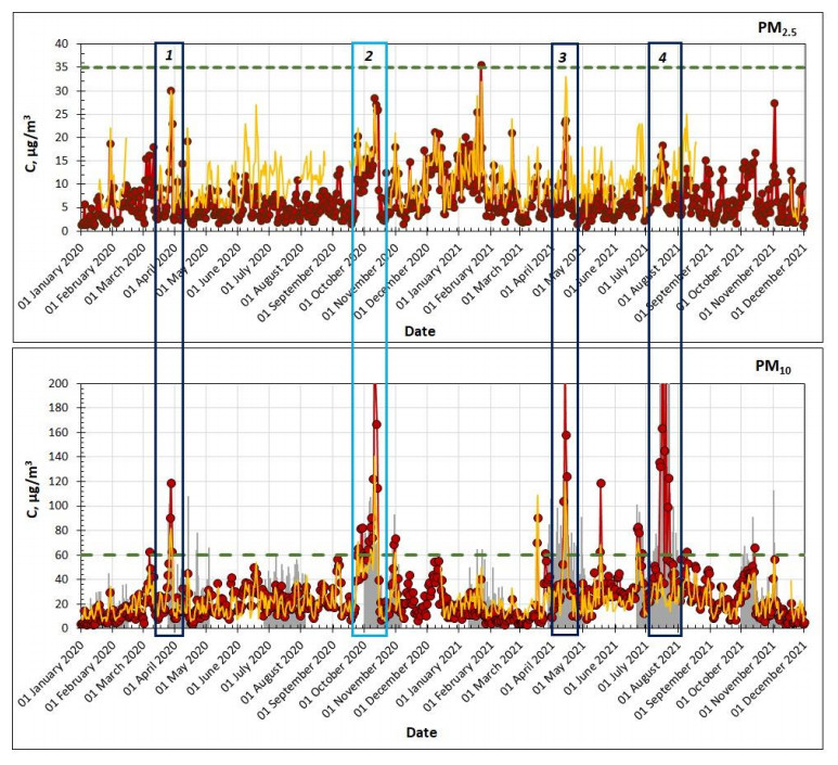
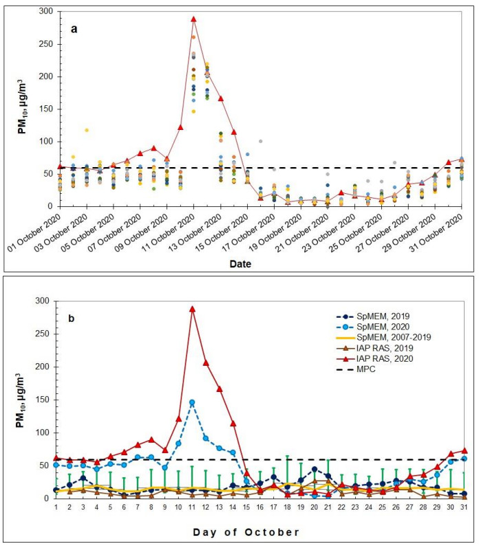
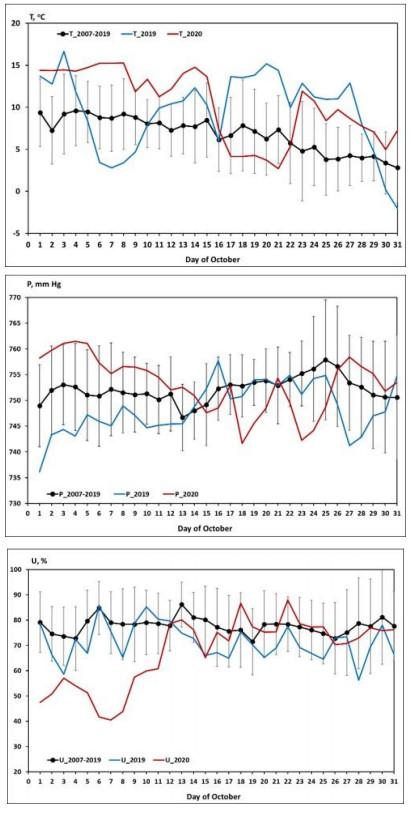
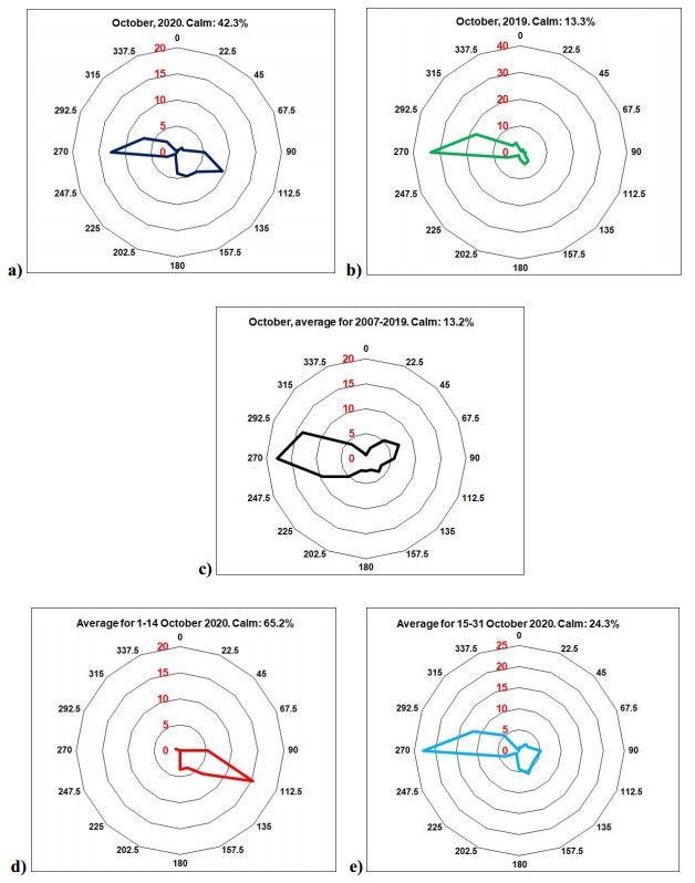
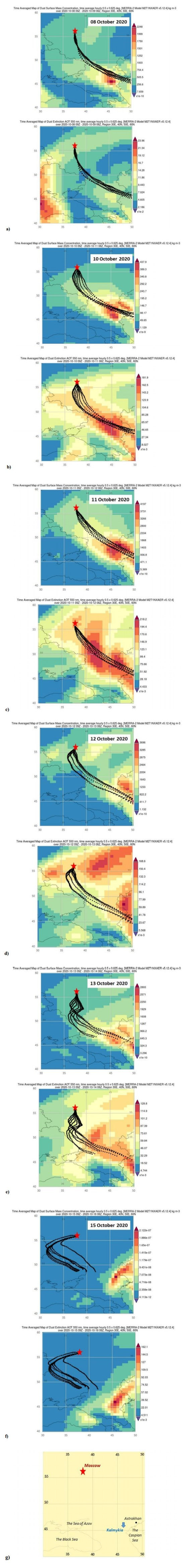
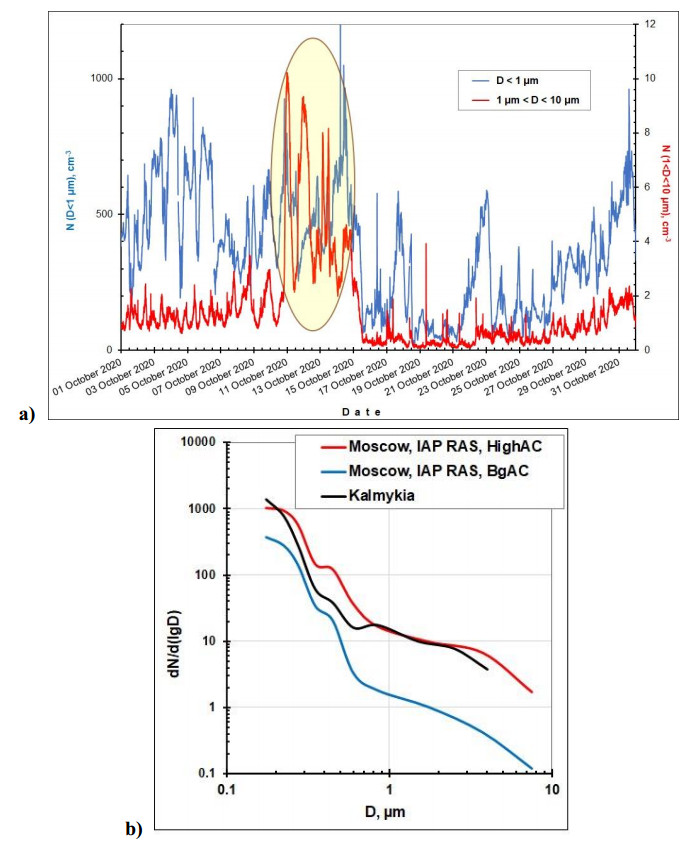
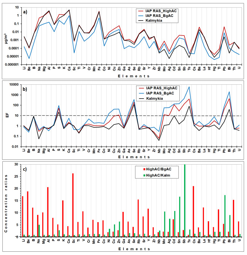
We analyzed the unique episode of long-range dust/sand atmospheric aerosol transport from the arid zones of the southern European territory of Russia, i.e. the Northern Caspian and Astrakhan regions and the Kalmykia Republic, to the Moscow region during fall 2020. Intensive complex experiments were carried out at the A.M. Obukhov Institute of Atmospheric Physics of the Russian Academy of Sciencesin the center of Moscow through different seasons during 2020–2021 to study the composition of near-surface aerosols in the Moscow megacity. The experimental data are considered to take into account the synoptic features and meteorological conditions. Abnormally high values of near-surface aerosol mass concentrations in Moscow were registered during the period from 6 to 14 of October 2020 under stable anti-cyclonic conditions, with calm or quiet/light wind (1–2 m/s), and under the conditions of the dominance of southeastern air mass transport. At the same time, the average daily mass concentration of aerosol particles PM10 exceeded the Maximum Permissible Concentration (MPC) value (60 µg/m3) by 1.5–4.5 times, and the number of large (micron) particles increased by an order or more. Comparative analysis of aerosol elemental composition in Moscow (during this episode) and in Kalmykia (according to observations in July 2020) showed high correlation for terrigenous elements' patterns. The aerosol origin for this episode was confirmed by performing long-range trajectory analysis of air mass transport (HYSPLIT model), and by using MERRA-2 reanalysis data for dust aerosol spatial distribution.
Citation: Dina Gubanova, Otto Chkhetiani, Anna Vinogradova, Andrey Skorokhod, Mikhail Iordanskii. Atmospheric transport of dust aerosol from arid zones to the Moscow region during fall 2020[J]. AIMS Geosciences, 2022, 8(2): 277-302. doi: 10.3934/geosci.2022017
We analyzed the unique episode of long-range dust/sand atmospheric aerosol transport from the arid zones of the southern European territory of Russia, i.e. the Northern Caspian and Astrakhan regions and the Kalmykia Republic, to the Moscow region during fall 2020. Intensive complex experiments were carried out at the A.M. Obukhov Institute of Atmospheric Physics of the Russian Academy of Sciencesin the center of Moscow through different seasons during 2020–2021 to study the composition of near-surface aerosols in the Moscow megacity. The experimental data are considered to take into account the synoptic features and meteorological conditions. Abnormally high values of near-surface aerosol mass concentrations in Moscow were registered during the period from 6 to 14 of October 2020 under stable anti-cyclonic conditions, with calm or quiet/light wind (1–2 m/s), and under the conditions of the dominance of southeastern air mass transport. At the same time, the average daily mass concentration of aerosol particles PM10 exceeded the Maximum Permissible Concentration (MPC) value (60 µg/m3) by 1.5–4.5 times, and the number of large (micron) particles increased by an order or more. Comparative analysis of aerosol elemental composition in Moscow (during this episode) and in Kalmykia (according to observations in July 2020) showed high correlation for terrigenous elements' patterns. The aerosol origin for this episode was confirmed by performing long-range trajectory analysis of air mass transport (HYSPLIT model), and by using MERRA-2 reanalysis data for dust aerosol spatial distribution.

| [1] | Seinfeld J, Pandis S (2006) Atmospheric Chemistry and Physics: From Air Pollution to Climate Change, 2nd Ed., New York: Wiley. |
| [2] |
Cess R, Potter G, Ghan S, et al. (1985) The climatic effects of large injections of atmospheric smoke and dust: A study of climate feedback mechanisms with one- and three-dimensional climate models. J Geophys Res 90: 12937–12950. https://doi.org/10.1029/JD090iD07p12937 doi: 10.1029/JD090iD07p12937

|
| [3] |
Schepanski K (2018) Transport of mineral dust and its impact on climate. Geosciences 8: 151. https://doi.org/10.3390/geosciences8050151 doi: 10.3390/geosciences8050151
|
| [4] |
Chaibou S, Ma A, Sha T (2020) Dust radiative forcing and its impact on surface energy budget over West Africa. Sci Rep 10: 12236. https://doi.org/10.1038/s41598-020-69223-4 doi: 10.1038/s41598-020-69223-4
|
| [5] | Budyko M, Golitsyn G, Izrael Y (1988) Global climatic catastrophes, Berlin, New York: Springer-Verlag. |
| [6] |
Brinkman A, McGregor J (1983) Solar radiation in dense Saharan aerosol in northern Nigeria. Quart J Roy Met Soc 109: 831–847. https://doi.org/10.1256/smsqj.46209 doi: 10.1256/smsqj.46209
|
| [7] | Gorchakova I, Mokhov I, Rublev A (2015) Radiation and temperature effects of the intensive injection of dust aerosol into the atmosphere. Izv Atmos Ocean Phys 51: 113–126. |
| [8] |
Hu ZY, Huang JP, Zhao C, et al. (2020) Modeling dust sources, transport, and radiative effects at different altitudes over the Tibetan Plateau. Atmos Chem Phys 20: 1507–1529. https://doi.org/10.5194/acp-20-1507-2020 doi: 10.5194/acp-20-1507-2020
|
| [9] |
Huang JP, Minnis P, Chen B, et al. (2008) Long-range transport and vertical structure of Asian dust from CALIPSO and surface measurements during PACDEX. J Geophys Res 113. https://doi.org/10.1029/2008JD010620 doi: 10.1029/2008JD010620
|
| [10] |
Yang L, Shi Z, Sun H, et al. (2021) Distinct effects of winter monsoon and westerly circulation on dust aerosol transport over East Asia. Theor Appl Climatol 144: 1031–1042. https://doi.org/10.1007/s00704-021-03579-z doi: 10.1007/s00704-021-03579-z
|
| [11] |
Vijayakumara K, Devara PCS, Vijaya Bhaskara Rao S, et al. (2016) Dust aerosol characterization and transport features based on combined ground-based, satellite and model-simulated data. Aeolian Res 21: 75–85. https://doi.org/10.1016/j.aeolia.2016.03.003 doi: 10.1016/j.aeolia.2016.03.003
|
| [12] |
Zayakhanov A, Zhamsueva G, Naguslaev S, et al. (2012) Spatiotemporal characteristics of the atmospheric AOD in the Gobi Desert according to data of the ground-based observations. Atmos Ocean Opt 25: 346–354. https://doi.org/10.1134/S1024856012050119 doi: 10.1134/S1024856012050119
|
| [13] |
Abdullaev S, Maslov V, Nazarov B, et al. (2015) The elemental composition of soils and dust aerosol in the south-central part of Tajikistan. Atmos Ocean Opt 28: 347–358. https://doi.org/10.1134/S1024856015040028 doi: 10.1134/S1024856015040028
|
| [14] |
Xiong J, Zhao T, Bai Y, et al. (2020) Climate characteristics of dust aerosol and its transport in major global dust source regions. J Atmos Sol-Terr Phys 209: 105415. https://doi.org/10.1016/j.jastp.2020.105415 doi: 10.1016/j.jastp.2020.105415
|
| [15] |
Ginoux P, Prospero J, Gill T, et al. (2012) Global-scale attribution of anthropogenic and natural dust sources and their emission rates based on MODIS Deep Blue aerosol products. Rev Geophys 50: RG3005. https://doi.org/10.1029/2012RG000388 doi: 10.1029/2012RG000388
|
| [16] |
Prospero J (1999) Long-range transport of mineral dust in the global atmosphere: Impact of African dust on the environment of the southeastern United States. PNAS 96: 3396–3403. https://doi.org/10.1073/pnas.96.7.3396 doi: 10.1073/pnas.96.7.3396
|
| [17] |
Maring H, Savoie D, Izaguirre M, et al. (2003) Mineral dust aerosol size distribution change during atmospheric transport. J Geophys Res 108: 8592. https://doi.org/10.1029/2002JD002536 doi: 10.1029/2002JD002536
|
| [18] |
Zhang YD, Cai YJ, Yu FQ, et al (2021) Seasonal variations and long-term trend of mineral dust aerosols over the Taiwan Region. Aerosol Air Qual Res 21: 200433. https://doi.org/10.4209/aaqr.2020.07.0433 doi: 10.4209/aaqr.2020.07.0433
|
| [19] |
Guedes A, Landulfo E, Montilla-Rosero E, et al. (2018) Detection of Saharan mineral dust aerosol transport over Brazilian northeast through a depolarization lidar. EPJ Web Conf 176: 05036. https://doi.org/10.1051/epjconf/201817605036 doi: 10.1051/epjconf/201817605036
|
| [20] |
Weinzierl B, Ansmann A, Prospero JM, et al. (2017) The Saharan aerosol long-range transport and aerosol–cloud-interaction experiment: Overview and selected highlights. BAMS 98: 1427–1451. https://doi.org/10.1175/BAMS-D-15-00142.1 doi: 10.1175/BAMS-D-15-00142.1
|
| [21] |
Does M, Knippertz P, Zschenderlein P, et al. (2018) The mysterious long-range transport of giant mineral dust particles. Sci Adv 4. https://doi.org/10.1126/sciadv.aau2768 doi: 10.1126/sciadv.aau2768
|
| [22] |
Asher EC, Christensen JN, Post A, et al. (2018) The transport of Asian dust and combustion aerosols and associated ozone to North America as observed from a mountaintop monitoring site in the California coast range. JGR Atmosphere 123: 4890–4909. https://doi.org/10.1029/2017JD028075 doi: 10.1029/2017JD028075
|
| [23] |
Akritidis D, Katragkou E, Georgoulias AK, et al. (2020) A complex aerosol transport event over Europe during the 2017 Storm Ophelia in CAMS forecast systems: Analysis and evaluation. Atmos Chem Phys 20: 13557–13578. https://doi.org/10.5194/acp-20-13557-2020 doi: 10.5194/acp-20-13557-2020
|
| [24] |
Ansmann A, Bösenberg J, Chaikovsky A, et al. (2003) Long-range transport of Saharan dust to northern Europe: The 11–16 October 2001 outbreak observed with EARLINET. J Geophys Res 108: 4783. https://doi.org/10.1029/2003JD003757 doi: 10.1029/2003JD003757
|
| [25] |
Conceição R, Silva HG, Mirão SJ, et al. (2018) Saharan dust transport to Europe and its impact on photovoltaic performance: A case study of soiling in Portugal. Sol Energy 160: 94–102. https://doi.org/10.1016/j.solener.2017.11.059 doi: 10.1016/j.solener.2017.11.059
|
| [26] |
Israelevich P, Ganor E, Alpert P, et al. (2012) Predominant transport paths of Saharan dust over the Mediterranean Sea to Europe. JGR Atmosphere 117: 2205. https://doi.org/10.1029/2011JD016482 doi: 10.1029/2011JD016482
|
| [27] |
Kaskaoutis D, Kosmopoulos G, Nastos P, et al. (2012) Transport pathways of Sahara dust over Athens, Greece as detected by MODIS and TOMS. Geomathematics Nat Hazards Risk 3: 35–54. https://doi.org/10.1080/19475705.2011.574296 doi: 10.1080/19475705.2011.574296
|
| [28] |
Pey J, Querol X, Alastuey A, et al. (2013) African dust outbreaks over the Mediterranean Basin during 2001–2011: PM10 concentrations, phenomenology and trends, and its relation with synoptic and mesoscale meteorology. Atmos Chem Phys 13: 1395–1410. https://doi.org/10.5194/acp-13-1395-2013 doi: 10.5194/acp-13-1395-2013
|
| [29] |
Salvador P, Artíñano B, Molero F, et al. (2013) African dust contribution to ambient aerosol levels across central Spain: Characterization of long-range transport episodes of desert dust. Atmos Res 127: 117–129. https://doi.org/10.1016/j.atmosres.2011.12.011 doi: 10.1016/j.atmosres.2011.12.011
|
| [30] |
Filonchyk M (2022) Characteristics of the severe March 2021 Gobi Desert dust storm and its impact on air pollution in China. Chemosphere 287: 132219. https://doi.org/10.1016/j.chemosphere.2021.132219 doi: 10.1016/j.chemosphere.2021.132219
|
| [31] |
Filonchyk M, Peterson M (2022) Development, progression, and impact on urban air quality of the dust storm in Asia in March 15–18, 2021. Urban Clim 41: 101080. https://doi.org/10.1016/j.uclim.2021.101080 doi: 10.1016/j.uclim.2021.101080
|
| [32] |
Filonchyk M, Hurynovich V (2020) Spatial distribution and temporal variation of atmospheric pollution in the South Gobi Desert, China, during 2016–2019. Environ Sci Pollut Res 27: 26579–26593. https://doi.org/10.1007/s11356-020-09000-y doi: 10.1007/s11356-020-09000-y
|
| [33] |
Guo JP, Lou MY, Miao YC, et al. (2017) Trans-Pacific transport of dust aerosols from East Asia: Insights gained from multiple observations and modeling. Environ Pollut 230: 1030–1039. https://doi.org/10.1016/j.envpol.2017.07.062 doi: 10.1016/j.envpol.2017.07.062
|
| [34] | Wu M, Liu X, Luo T, et al. (2017) Trans-Pacific transport of Asian dust: The CESM model analysis and comparison with satellite observations. Amer Geophys Union. Available from: https://ui.adsabs.harvard.edu/abs/2017AGUFM.A33F2441W/abstract |
| [35] |
Yumimoto K, Eguchi K, Uno IR, et al. (2010) Summertime trans-Pacific transport of Asian dust. Geophys Res Lett 37. https://doi.org/10.1029/2010GL043995 doi: 10.1029/2010GL043995
|
| [36] |
Han Y, Fang X, Zhao T, et al. (2008) Long range trans-Pacific transport and deposition of Asian dust aerosols. J Environ Sci 20: 424–428. https://doi.org/10.1016/s1001-0742(08)62074-4 doi: 10.1016/s1001-0742(08)62074-4
|
| [37] |
Wuebbles DJ, Lei H, Lin JT (2007) Intercontinental transport of aerosols and photochemical oxidants from Asia and its consequences. Environ Pollut 150: 65–84. https://doi.org/10.1016/j.envpol.2007.06.066 doi: 10.1016/j.envpol.2007.06.066
|
| [38] |
Huang Z, Huang J, Hayasaka T, et al. (2015) Short-cut transport path for Asian dust directly to the Arctic: A case study. Environ Res Lett 10: 114018. https://doi.org/10.1088/1748-9326/10/11/114018 doi: 10.1088/1748-9326/10/11/114018
|
| [39] | Kondratyev I, Kachur A, Yurchenko S, et al. (2005) Synoptic and geochemical aspects of abnormal dust transfer in south Primorskii krai. Vestn Far East Branch Russ Acad Sci 3: 55–65. (In Russian) |
| [40] |
Kalinskaya D, Papkova A, Varenik A (2021) The case of absorbing aerosol anomalous transport over the Black Sea in the spring of 2020. Sovr Probl DZZ Kosm 18: 287–298. (In Russian). https://doi.org/10.21046/2070-7401-2021-18-2-287-298 doi: 10.21046/2070-7401-2021-18-2-287-298
|
| [41] |
Kutuzov S, Mikhalenko V, Shahgedanova M, et al. (2014) Ways of far-distance dust transport onto Caucasian glaciers and chemical composition of snow on the Western plateau of Elbrus. Ice Snow 54: 5–15. (In Russian). https://doi.org/10.15356/2076-6734-2014-3-5-15 doi: 10.15356/2076-6734-2014-3-5-15
|
| [42] |
Sokhi R, Singh V, Querolet X, et al. (2021) A global observational analysis to understand changes in air quality during exceptionally low anthropogenic emission conditions. Environ Intern 157: 106818. https://doi.org/10.1016/j.envint.2021.106818 doi: 10.1016/j.envint.2021.106818
|
| [43] | Mosecomonitoring. Measuring stations. Available from: https://mosecom.mos.ru/measuring-stations/ |
| [44] | Ogorodnikov B (1996) Parameters of aerosols in the atmospheric boundary layer over Moscow. Izv RAN Fizika Atmosfery i Okeana 32: 163–171. (In Russian) |
| [45] |
Gubanova DP, Belikov IB, Elansky NF, et al. (2018) Variations in PM2.5 surface concentration in Moscow according to observations at MSU meteorological observatory. Atmos Ocean Opt 31: 290–299. https://doi.org/10.1134/S1024856018030065 doi: 10.1134/S1024856018030065
|
| [46] |
Trefilova AV, Artamonova MS, Kuderina TM, et al. (2013) Chemical composition and microphysical characteristics of atmospheric aerosol over Moscow and its vicinity in June 2009 and during the fire peak of 2010. Izv Atmos Ocean Phys 49: 765–778. https://doi.org/10.1134/S0001433813070062 doi: 10.1134/S0001433813070062
|
| [47] |
Kasimov N, Vlasov DV, Kosheleva NE (2020) Enrichment of road dust particles and adjacent environments with metals and metalloids in eastern Moscow. Urban Clim 32: 100638. https://doi.org/10.1016/j.uclim.2020.100638 doi: 10.1016/j.uclim.2020.100638
|
| [48] |
Chubarova N, Androsova Y, Lezina Y (2021) The dynamics of the atmospheric pollutants during the Covid-19 pandemic 2020 and their relationship with meteorological conditions in Moscow. GES 14: 168–182. https://doi.org/10.24057/2071-9388-2021-012 doi: 10.24057/2071-9388-2021-012
|
| [49] |
Gubanova DP, Elansky NF, Skorokhod AI, et al. (2020) Physical and chemical properties of atmospheric aerosols in Moscow and its suburb for climate assessments. IOP Conf Ser Earth Environ Sci 606: 012019. https://doi.org/10.1088/1755-1315/606/1/012019 doi: 10.1088/1755-1315/606/1/012019
|
| [50] |
Gubanova DP, Iordanskii MA, Kuderina TM, et al. (2021) Elemental composition of aerosols in the ground air of Moscow: Seasonal changes in 2019 and 2020. Atmos Ocean Opt 34: 475–482. https://doi.org/10.1134/S1024856021050122 doi: 10.1134/S1024856021050122
|
| [51] |
Shukurov K, Shukurova L (2019) Aral's potential sources of dust for Moscow region. E3S Web Conf 99: 02015. https://doi.org/10.1051/e3sconf/20199902015 doi: 10.1051/e3sconf/20199902015
|
| [52] |
Shukurov KA, Shukurova LM (2017) Source regions of ammonium nitrate, ammonium sulfate, and natural silicates in the surface aerosols of Moscow oblast. Izv Atmos Ocean Phys 53: 316–325. https://doi.org/10.1134/S0001433817030136 doi: 10.1134/S0001433817030136
|
| [53] |
Shukurov K, Chkhetiani O (2017) Probability of transport of air parcels from the arid lands in the southern Russia to Moscow region. Proc SPIE 10466. https://doi.org/10.1117/12.2287932 doi: 10.1117/12.2287932
|
| [54] | HYSPLIT. Available from: www.arl.noaa.gov |
| [55] | MERRA-2. Available from: https://giovanni.gsfc.nasa.gov/giovanni/ |
| [56] | Erhardt H (1985) Rentgenofluorescentnyj Analiz. Primenenie v Zavodskih Laboratorijah, Moscow: Metallurgija. (In Russian). |
| [57] | Kudryashov V (1997) Analysis of the elemental composition atmospheric aerosols by physical methods. In Problemy Fiziki Atmosfery: Mezhvuzovskii Sbornik[Problems of Atmospheric Physics: Interuniversity Transactions], Saint-Petersburg: SPbGU, 97–130. (In Russian) |
| [58] | Karandashev V, Turanov A, Orlova T, et al. (2007) Use of mass spectrometry with inductively coupled plasma method for element analysis of surrounding medium objects. Russ Zavod Lab Diagn Mater 73: 12–22. (In Russian). Available from: https://www.elibrary.ru/item.asp?id=9470754 |
| [59] | Reliable prognosis. (In Russian). Available from: https://rp5.ru |
| [60] | Windy. (In Russian). Available from: https://www.windy.com/ru. |
| [61] | Weatherarchive. (In Russian). Available from: http://weatherarchive.ru/Pogoda/Moscow. |
| [62] |
Gubanova DP, Vinogradova AA, Iordanskii MA, et al. (2021) Time variations in the composition of atmospheric aerosol in Moscow in spring 2020. Izv Atmos Ocean Phys 57: 297–309. https://doi.org/10.1134/S0001433821030051 doi: 10.1134/S0001433821030051
|
| [63] |
Gubanova DP, Vinogradova AA, Iordanskii MA, et al. (2022) Variability of near-surface aerosol composition in Moscow in 2020–2021: Episodes of extreme air pollution of different genesis. Atmosphere 13: 574. https://doi.org/10.3390/atmos13040574 doi: 10.3390/atmos13040574
|
| [64] |
Gubanova DP, Vinogradova AA, Skorokhod A, et al. (2021) Abnormal aerosol air pollution in Moscow near the local anthropogenic source in July 2021. Hydrometeorological Res Forecast 4: 134–148. https://doi.org/10.37162/2618-9631-2021-4-134-148 doi: 10.37162/2618-9631-2021-4-134-148
|
| [65] | Vinogradov A (1962) Srednie soderzhaniya khimicheskikh elementov v glavnykh tipakh izverzhennykh gornykh porod zemnoy kory[Average content of chemical elements in major types of erupted rocks of the Earth crust]. Geokhimiya [Geochemistry] 7: 555–571. |
| [66] | Kasimov NS, Vlasov DV, Kosheleva NE, et al. (2016) Geochemistry of landscapes of eastern Moscow, Moscow: APR. (In Russian). |
Figures(7) / Tables(1)

Dina Gubanova, Otto Chkhetiani, Anna Vinogradova, Andrey Skorokhod, Mikhail Iordanskii. Atmospheric transport of dust aerosol from arid zones to the Moscow region during fall 2020[J]. AIMS Geosciences, 2022, 8(2): 277-302. doi: 10.3934/geosci.2022017


 DownLoad: