In this paper, I introduce a comprehensive workflow aimed at optimizing oil production and CO2 geological storage. I show that the same methodology can be applied to different categories of problems: a) real-time reservoir fluid mapping for predicting and delaying water breakthrough time as far as possible in oil production; b) real-time CO2 mapping for maximizing the sweep efficiency and storage capacity of CO2 in geological formations. Despite their intrinsic differences, these types of problems share common aspects, issues and possible solutions. In both cases, various geophysical techniques can be applied, including Electric Resistivity Tomography (briefly ERT) for accurate fluid mapping and monitoring. This method is highly effective and sensitive for detecting the type of fluid and for estimating saturation in the geological formations. The robustness and the accuracy of the ERT models increase if densely spaced electrodes layouts are permanently deployed into the production and injection wells. In the first part of the paper, I discuss how in both scenarios of oil production and CO2 storage, we can apply time-lapse borehole ERT method for mapping fluids in the reservoir. Next, I discuss how to apply various techniques of time-series analysis for predicting the evolution of the fluids distribution over time. Finally, using Q-Learning, that is a specific Reinforcement Learning method, I discuss how we can optimize the decisional workflow using our models about past, real-time and predicted fluids displacement. The result is the definition of a "best policy" addressed to both problems of optimized oil production and safe CO2 geological storage. In the second part of the paper, I show benefits and limitations of my approach with the support of synthetic tests.
Citation: Paolo Dell'Aversana. Reservoir prescriptive management combining electric resistivity tomography and machine learning[J]. AIMS Geosciences, 2021, 7(2): 138-161. doi: 10.3934/geosci.2021009
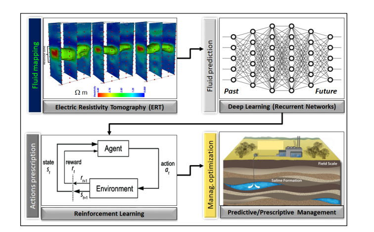
In this paper, I introduce a comprehensive workflow aimed at optimizing oil production and CO2 geological storage. I show that the same methodology can be applied to different categories of problems: a) real-time reservoir fluid mapping for predicting and delaying water breakthrough time as far as possible in oil production; b) real-time CO2 mapping for maximizing the sweep efficiency and storage capacity of CO2 in geological formations. Despite their intrinsic differences, these types of problems share common aspects, issues and possible solutions. In both cases, various geophysical techniques can be applied, including Electric Resistivity Tomography (briefly ERT) for accurate fluid mapping and monitoring. This method is highly effective and sensitive for detecting the type of fluid and for estimating saturation in the geological formations. The robustness and the accuracy of the ERT models increase if densely spaced electrodes layouts are permanently deployed into the production and injection wells. In the first part of the paper, I discuss how in both scenarios of oil production and CO2 storage, we can apply time-lapse borehole ERT method for mapping fluids in the reservoir. Next, I discuss how to apply various techniques of time-series analysis for predicting the evolution of the fluids distribution over time. Finally, using Q-Learning, that is a specific Reinforcement Learning method, I discuss how we can optimize the decisional workflow using our models about past, real-time and predicted fluids displacement. The result is the definition of a "best policy" addressed to both problems of optimized oil production and safe CO2 geological storage. In the second part of the paper, I show benefits and limitations of my approach with the support of synthetic tests.

| [1] | Chaperon I (1986) Theoretical Study of Coning Toward Horizontal and Vertical Wells in Anisotropic Formations: Subcritical and Critical Rates. SPE Annu Tech Conf Exhib, 5-8. |
| [2] |
Chierici GL, Ciucci GM, Pizzi G (1964) A Systematic Study of Gas and Water Coning By Potentiometric Models. J Pet Technol 16: 923-929. doi: 10.2118/871-PA

|
| [3] | Wheatley MJ (1985) An Approximate Theory of Oil/Water Coning. SPE Annual Technical Conference and Exhibition, Las Vegas, Nevada, USA, 22-26. |
| [4] | Al-Sikaiti SH, Regtien J (2008) Challenging Conventional Wisdom, Waterflooding Experience on Heavy Oil Fields in Southern Oman. World Heavy Oil Congr: 10-12. |
| [5] |
Karami M, Khaksar Manshad A, Ashoori S (2014) The Prediction of Water Breakthrough Time and Critical Rate with a New Equation for an Iranian Oil Field. Pet Sci Technol 32: 211-216. doi: 10.1080/10916466.2011.586960
|
| [6] |
Jiang X (2011) A review of physical modelling and numerical simulation of long-term geological storage of CO2. Appl Energy 88: 3557-3566. doi: 10.1016/j.apenergy.2011.05.004
|
| [7] |
Jung JY, Huh C, Kang SG, et al. (2013) CO2 transport strategy and its cost estimation for the offshore CCS in Korea. Appl Energy 111: 1054-1060. doi: 10.1016/j.apenergy.2013.06.055
|
| [8] | Buscheck TA, White JA, Chen M, et al. (2014) Pre-injection brine production for managing pressure in compartmentalized CO2 storage reservoirs. Energy Procedia 63, 5333-5340. |
| [9] |
González-Nicolás A, Cihan A, Petrusak R, et al. (2019) Pressure management via brine extraction in geological CO2 storage: Adaptive optimization strategies under poorly characterized reservoir conditions. Int J Greenhouse Gas Control 83: 176-185. doi: 10.1016/j.ijggc.2019.02.009
|
| [10] | Pongtepupathum W, Williams J, Krevor S, et al. (2017) Optimising Brine Production for Pressure Management During CO2 sequestration in the Bunter Sandstone of the UK Southern North Sea. Soc Pet Eng. |
| [11] | Tarrahi M, Afra S (2015) Optimization of Geological Carbon Sequestration in Heterogeneous Saline Aquifers through Managed Injection for Uniform CO2 Distribution. Carbon Management Technology Conference. |
| [12] |
Liao C, Liao X, Mu L, et al. (2017) Improving water-alternating-CO2 flooding of heterogeneous, low permeability oil reservoirs using ensemble optimisation algorithm. Int J Global Warming 12: 242-260. doi: 10.1504/IJGW.2017.084509
|
| [13] | Shamshiri H, Jafarpour B (2010) Optimization of Geologic CO2 Storage in Heterogeneous Aquifers Through Improved Sweep Efficiency. SPE International Conference on CO2 Capture, Storage, and Utilization held in New Orleans, Louisiana, 10-12. |
| [14] | Kazakis N, Pavlou A, Vargemezis G, et al. (2016) Seawater intrusion mapping using electrical resistivity tomography and hydrochemical data. An application in the coastal area of eastern Thermaikos Gulf, Greece. Sci Total Environ 543: 373-387. |
| [15] | Goldman M, Kafri U (2006) Hydrogeophysical applications in coastal aquifers. In: Vereecken H, Author, Applied Hydrogeophysics, Eds., Springer: Dordrecht, The Netherlands, 233-254. |
| [16] | Kuras O, Pritchard J, Meldrum P, et al. (2009) Monitoring hydraulic processes with automated time-lapse electrical resistivity tomography (ALERT): Compt Rendus Geosci 341: 868-885. |
| [17] | Dell'Aversana P, Rizzo E, Servodio R (2017) 4D borehole electric tomography for hydrocarbon reservoir monitoring. EAGE Conference and Exhibition, 2017: 1-5. |
| [18] | McNeice GW, Colombo D (2018) 3D inversion of surface to borehole CSEM for waterflood monitoring. SEG Int Expo Ann Meet, 878-880. |
| [19] | Bergmann P, Schmidt-Hattenberger C, Kiessling D, et al. (2012) Surface-downhole electrical resistivity tomography applied to monitoring of CO2 storage at Ketzin, Germany. Geophysics 77: B253-B267. |
| [20] |
Bergmann P, Schmidt-Hattenberger C, Labitzke1 T, et al. (2017) Fluid injection monitoring using electrical resistivity tomography—five years of CO2 injection at Ketzin, Germany. Geophys Prospect 65: 859-875. doi: 10.1111/1365-2478.12426
|
| [21] |
Schmidt-Hattenberger C, Bergmann P, Bö sing D, et al. (2013) Electrical resistivity tomography (ERT) for monitoring of CO2 migration-from tool development to reservoir surveillance at the Ketzinpilot site. Energy Procedia 37: 4268-4275. doi: 10.1016/j.egypro.2013.06.329
|
| [22] |
Descloitres M, Ribolzi O, Le Troquer Y (2003) Study of infiltration in a Sahelian gully erosion area using time-lapse resistivity mapping. Catena 53: 229-253. doi: 10.1016/S0341-8162(03)00038-9
|
| [23] | Dell'Aversana P, Servodio R, Bottazzi F, et al. (2019_a) Asset Value Maximization through a Novel Well Completion System for 3d Time Lapse Electromagnetic Tomography Supported by Machine Learning. Abu Dhabi Int Pet Exhib Conf. |
| [24] | Dell'Aversana P, Servodio R, Bottazzi F, et al, (2019_b). Asset Value Maximization through a Novel Well Completion System for 3d Time Lapse Electromagnetic Tomography Supported by Machine Learning. Soc Pet Eng J. |
| [25] | Bottazzi F, Dell'Aversana P, Molaschi C, et al. (2020) A New Downhole System for Real Time Reservoir Fluid Distribution Mapping: E-REMM, the Eni-Reservoir Electro-Magnetic Mapping System. Int Pet Technol Conf. |
| [26] | Brown RG (1956) Exponential Smoothing for Predicting Demand. Cambridge, Massachusetts: Arthur D. Little Inc 15. |
| [27] |
Saad EW, Prokhorov DV, Wunsch DC (1998) Comparative study of stock trend prediction using time delay, recurrent and probabilistic neural networks. IEEE T Neural Network 9: 1456-1470. doi: 10.1109/72.728395
|
| [28] |
Tealab A (2018) Time series forecasting using artificial neural networks methodologies: A systematic review. Future Comput Inform J 3: 334-340. doi: 10.1016/j.fcij.2018.10.003
|
| [29] |
Sherstinsky A (2020) Fundamentals of Recurrent Neural Network (RNN) and Long Short-Term Memory (LSTM) Network. Phys D 404: 132306. doi: 10.1016/j.physd.2019.132306
|
| [30] |
Kaelbling LP, Littman ML, Moore AW (1996) Reinforcement Learning: A Survey. J Artif Intell Res 4: 237-285. doi: 10.1613/jair.301
|
| [31] | Raschka S, Mirjalili V (2017) Python Machine Learning: Machine Learning and Deep Learning with Python, scikit-learn, and TensorFlow, 2nd Ed., PACKT Books. |
| [32] | Russell S, Norvig P (2016) Artificial Intelligence: A Modern approach, Global Edition, Pearson Education, Inc., publishing as Prentice Hall. |
| [33] | Machine learning workflows. Multidisciplinary applications using Python, 2021. Available from: https://www.researchgate.net/publication/348741974_Q_Learning_generic. |
| [34] |
Benson SM, Surles T (2006) Carbon dioxide capture and storage: an overview with emphasis on capture and storage in deep geological formations. Proc IEEE 94: 1795-1805. doi: 10.1109/JPROC.2006.883718
|
| [35] |
Christensen NB, Sherlock D, Dodds K (2006) Monitoring CO2 injection with cross-hole electrical resistivity tomography. Explor Geophys 37: 44-49. doi: 10.1071/EG06044
|
| [36] |
LaBrecque DJ, Miletto M, Daily W, et al. (1996) The effects of noise on Occam's inversion of resistivity tomography data. Geophysics 61: 538-548. doi: 10.1190/1.1443980
|
| [37] | Dell'Aversana P, Carbonara S, Vitale S, et al (2011) Quantitative estimation of oil saturation from marine CSEM data: A case history. First Break 29. |
| [38] | Befus KM (2017) Pyres: A Python Wrapper for Electrical Resistivity Modeling with R2. J Geophys Eng 15. |
| [39] | Binley A, A Kemna (2005) Electrical Methods, In: Hydrogeophysics by Rubin and Hubbard Eds., Springer, 129-156. |
| [40] | Binley A (2015) Tools and Techniques: DC Electrical Methods, In: Treatise on Geophysics, 2nd Ed., Schubert: Elsevier, 233-259. |
| [41] | Binley A (2016) R2 version 3.1 Manual. Lancaster, UK. Available from: http://es.lancs.ac.uk/people/amb/Freeware/freeware.htm. |
| [42] | PUNQ-S3 reservoir model, Imperial College of London. Available from: https://www.imperial.ac.uk/earth-science/research/research-groups/perm/standard-models/. |
| [43] | Archie GE (1950) Introduction to petrophysics of reservoir rocks. AAPG Bulletin 34: 943-961. |
| [44] |
Claerbout JF, Muir F (1973) Robust modeling with erratic data. Geophysics 18: 826-844. doi: 10.1190/1.1440378
|
| [45] |
Sagheer A, Kotb M (2019) Time series forecasting of petroleum production using deep LSTM recurrent networks. Neurocomputing 323: 203-213. doi: 10.1016/j.neucom.2018.09.082
|


Figures(16) / Tables(2)

Paolo Dell'Aversana. Reservoir prescriptive management combining electric resistivity tomography and machine learning[J]. AIMS Geosciences, 2021, 7(2): 138-161. doi: 10.3934/geosci.2021009


 DownLoad: