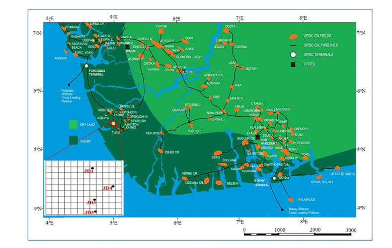
Figure 1.
Map of Niger Delta showing the location of study and oil production sites [21].
Citation: O. A. Oluwadare, M.T. Olowokere, F. Taoili, P.A. Enikanselu, R.M. Abraham-Adejumo. Application of time-frequency decomposition and seismic attributes for stratigraphic interpretation of thin reservoirs in 'Jude Field', Offshore Niger Delta[J]. AIMS Geosciences, 2020, 6(3): 378-396. doi: 10.3934/geosci.2020021
| [1] | Yasir Bashir, Muhammad Afiq Aiman Bin Zahari, Abdullah Karaman, Doğa Doğan, Zeynep Döner, Ali Mohammadi, Syed Haroon Ali . Artificial intelligence and 3D subsurface interpretation for bright spot and channel detections. AIMS Geosciences, 2024, 10(4): 662-683. doi: 10.3934/geosci.2024034 |
| [2] | Li Ding, Yubing Wu, Xuechao Liu, Fenfen Liu, Harry Mei . Application of Microbial Geochemical Exploration Technology in Identifying Hydrocarbon Potential of Stratigraphic Traps in Junggar Basin, China. AIMS Geosciences, 2017, 3(4): 576-589. doi: 10.3934/geosci.2017.4.576 |
| [3] | Anthony I Nzekwu, Richardson M Abraham-A . Reservoir sands characterisation involving capacity prediction in NZ oil and gas field, offshore Niger Delta, Nigeria. AIMS Geosciences, 2022, 8(2): 159-174. doi: 10.3934/geosci.2022010 |
| [4] | Khalid Ahmad, Umair Ali, Khalid Farooq, Syed Kamran Hussain Shah, Muhammad Umar . Assessing the stability of the reservoir rim in moraine deposits for a mega RCC dam. AIMS Geosciences, 2024, 10(2): 290-311. doi: 10.3934/geosci.2024017 |
| [5] | Tofig R. Akhmedov . 3D seismic survey data processing and interpretation by use of latest tools applied for discovery of new traps in Pleistocene deposits of Hovsan field. AIMS Geosciences, 2021, 7(1): 95-112. doi: 10.3934/geosci.2021005 |
| [6] | Lev Eppelbaum . Processing and interpretation of magnetic data in the Caucasus Mountains and the Caspian Sea: A review. AIMS Geosciences, 2024, 10(2): 333-370. doi: 10.3934/geosci.2024019 |
| [7] | Eduardo Antonio Rossello . Effects of the Guando Slump on the tectonic interpretation of the Boquerón Thrust in the Guando oilfield [Tolima, Colombia]. AIMS Geosciences, 2025, 11(2): 370-386. doi: 10.3934/geosci.2025016 |
| [8] | Maria C. Mariani, Hector Gonzalez-Huizar, Masum Md Al Bhuiyan, Osei K. Tweneboah . Using Dynamic Fourier Analysis to Discriminate Between Seismic Signals from Natural Earthquakes and Mining Explosions. AIMS Geosciences, 2017, 3(3): 438-449. doi: 10.3934/geosci.2017.3.438 |
| [9] | Ariane Locat, Pascal Locat, Hubert Michaud, Kevin Hébert, Serge Leroueil, Denis Demers . Geotechnical characterization of the Saint-Jude clay, Quebec, Canada. AIMS Geosciences, 2019, 5(2): 273-302. doi: 10.3934/geosci.2019.2.273 |
| [10] | Pezhman Soltani Tehrani, Hamzeh Ghorbani, Sahar Lajmorak, Omid Molaei, Ahmed E Radwan, Saeed Parvizi Ghaleh . Laboratory study of polymer injection into heavy oil unconventional reservoirs to enhance oil recovery and determination of optimal injection concentration. AIMS Geosciences, 2022, 8(4): 579-592. doi: 10.3934/geosci.2022031 |
To find out the prospect in the seismic data, it ought to bear a striking resemblance to geological cross-sections which makes interpretation easy. In the absence of this, geological interpretation of the seismic data is done based on knowledge of the basic principles. Most especially when it is within complex by-passed zones with subtle structures and the bandwidth of the data is not supportive of the interpretation. Previous researchers have used spectral decomposition technique on seismic data as an interpretation tool for direct hydrocarbon indication, investigation of attenuation effects produced by hydrocarbon and also for thickness estimation.
Partyka et al. applied spectral decomposition to seismic data to image thickness changes and delineate channels [1]. Marfurt and Kirlin also used the Discrete Fourier Transform to map time thicknesses i.e. estimating bed thickness via time difference between the peak and the trough of the seismic response [2]. Castagna et al. and Sinha et al. applied spectral decomposition as a direct-hydrocarbon indicator [3,4]. Tomasso et al. used spectral re-composition to recover the frequencies and its associated amplitudes (weights) as a reversed problem by an improved formula [5]. This proved to be a potent way of characterizing stratigraphic models using sensitivity analysis, unicity and stability. Distinct measurements or quantities obtained directly from the seismic data are used in seismic interpretation. These quantities are referred to as seismic attributes. Other subtle or hidden information which is unique can be derived from these attributes. The information could be used to detect, characterize, predict and keep under surveillance the hydrocarbon reservoirs [6,7]. The major attribute used in seismic interpretation is the amplitude, though its interpretation in thin-bedded reservoirs is a bit complicated [8]. The measurements can either be done on the reflection amplitude data, data along specific horizons or on the transformed data. Within certain frequency band, hidden and subtle structures become visible because of the effect of tuning. The attributes are important in solving the difficulty of characterization of thin layers.
Abdel-Fatah et al. used seismic attributes to illustrate different structural features that played important roles in the hydrocarbon potentialities and prospect identification of the Aptian Alamein Dolomite rock within the Razzak oil field in the northern part of Abu Gharadig Basin (Western Desert of Egypt) [9]. Fadul et al. also used seismic attributes for seismic interpretation of the tectonic regime of Sudanese Rift system and the implications of hydrocarbon exploration in “Neem Field”, Muglad Basin [10]. Most of this approach have used one or two of the various types of wavelet transformation technique, mostly within low-frequency bandwidth as a probable hydrocarbon-bearing zone.
Little work has been done using high frequency to probe deeper to unobvious structures with a reasonable proportion of hydrocarbon. The low frequency with longer wavelength penetrates better for thick reservoirs but the high frequency with short-wavelength probes deeper for a thinly bedded reservoir. Since seismic data is band limited and has a limited vertical resolution, seismic may not detect subtle structures especially when the structure is complex. The seismic data in time has to be converted to discreet frequencies or wavenumber using Spectral decomposition. In other words, it’s the use of small or short windows for transforming and displaying frequency/wavenumber spectra [11]. Spectral decomposition can be done by using different methods such as short window discreet Fourier transform, Continuous wavelet transform, stock-well transform, matching pursuit or by using Fast Fourier Transform [12,13]. The individual technique has its edge and flaws. Discrete Fourier Transform (DFT), Short Time Fourier Transform (STFT) and Fast Fourier Transform (FFT) make use of windows which has an intense consequence on the vertical resolution of the output. According to [12], STFT involves using windowed function transform discreet time series to its corresponding frequency domain. The disadvantage of STFT is that it makes use of a fixed analysis window. When a window function is chosen for STFT, the time-frequency resolution becomes fixed over the continuous time-frequency spectrum analysis [14]. For a function with a long period, minute changes in the time domain become indeterminate. In CWT, the frequency dispensation of non- stationary time series is examined. Unlike STFT, CWT does not use have fixed time-frequency resolution for its analysis. The frequency varies with the window size but when the frequency is low, events that are tightly spaced becomes unresolvable [4]. Also, the ringing effect associated with this approach due to poor signal makes it unsuitable for seismic data in some cases.
Fast Fourier Transform is a robust method in spectral decomposition because of its efficiency in resolving high-frequency events and the fact that it computes the same result more quickly. The difference in speed is enormous, most especially for long set data which may be in thousands or millions. The time taken for computation can also be reduced tremendously by several orders of magnitude. In FFT, for a function within a period, small changes are easily observed. This enhances stratigraphic features by showing variation in thickness from stratigraphic attributes. The spectral is enhanced to maximize the average frequency as well as the bandwidth by improving the resolution and providing direct attributes for reservoir model as it combines several data. The effect of earth absorption and wavelet overprint are removed from seismic data through spectral decomposition technique while the resolution is enhanced.
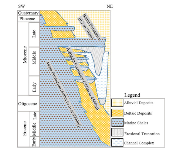
The Niger delta basin is one of the largest subaerial basins in Africa. The basin is assumed to have emerged from a failed rift junction due to the separation of the South American and African plates in the late Jurassic to mid-Cretaceous [15]. The structural and stratigraphic styles used to predict the availability of hydrocarbons in place are directly related to different events of geologic formation. “Jude Field” is located in the Offshore Depobelt of the basin within latitude 5.2°N and 5.6°N and longitude 4.2°E and 4.8°E (Figure 1). The emergence of the Niger Delta basin is as a result of series of events. According to [16], the regular pattern of long-shore currents resulted in the geomorphology of the Niger Delta coast. The Niger Delta consists of the regressive wedge of clastic sediments of maximum thickness of about 12 km [17]. The Delta is divided into three subsurface lithostratigraphic units. These are the major transgressive marine Akata Shale, the petroliferous parallic Agbada Formation, and the continental Benin Sands [18]. They represent pro-grading depositional facies that are distinguished mostly based on sand-shale ratios [17,19,20]. The three sedimentary sequences are tertiary in age (Figure 2). The Benin Formation which is the youngest consists predominantly of massive, highly porous fresh water-bearing sandstone with local interbed of shale [18]. Very little hydrocarbon accumulation has been associated with it. The Benin Formation is underlain by the Agbada Formation which consists of alternating sandstones and shale and it is of fluvio-marine origin. The age is from Eocene in the north to Pliocene in the south. The thickness is about 300 m to a maximum thickness of 4500 m. The Akata Formation underlies the Agbada Formation and it is the oldest. It consists of shale with inter-bedding of sands and siltstones. It is of the typical marine environment with a maximum thickness of about 6100 m.
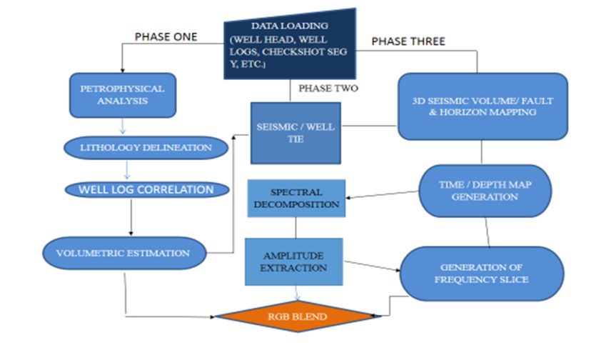
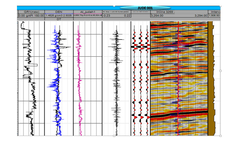
Structural and stratigraphic interpretation of 3D seismic data for reservoir characterization in an area with intense faulting such as Niger Delta is typically difficult and strongly model-driven. An integrated approach is used for better understanding of the geology and to enhance the interpretation (Figure 3). Details on the petrophysics are not given here due to the objective of this study. Firstly, well to seismic tie is carried out to ensure that the horizons picked on the seismic sections are true representatives of the ones picked on well logs from the good correlation panel. Also, it is used to correct for a shift in time in the log signature concerning time. From the data, the gamma-ray log was extracted from the suite of logs of well 1 within the depth range of interest. This was placed on a section using check-shot survey data and used for the time-depth conversion. To bridge the geological information both in time (seismic) and depth (well data), synthetic seismogram is generated. This involves time conversion of the measurements obtained in wells (depth) using the check-shot and sonic logs or generating synthetic seismogram from density and sonic logs, and a seismic wavelet by calculating reflection coefficients and acoustic impedance which are convolved using a wavelet (Figure 4). By generating a synthetic seismogram based on petrophysics, it is possible to identify the origin of seismic reflectors and trace them laterally along the seismic line.


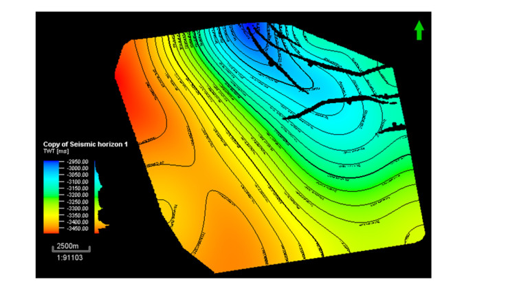
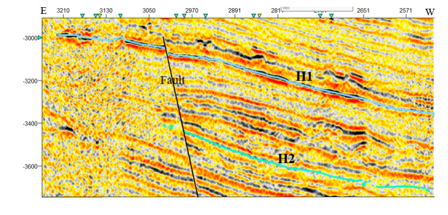
Two marker horizons were mapped and interpreted along with the thin reflectors and correlating across faults.
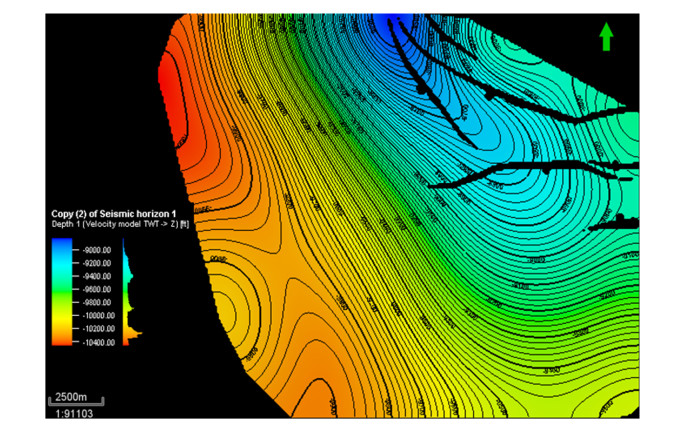
The horizons are AJ2 and BJ2, representing the first and second respectively. The results of the interpretation were presented as maps, time (Figure 5) and depth structural maps (Figure 6) for both horizons.


Oftentimes, layers within clastic rocks have a thickness below the resolution of the dominant frequencies of the seismic data. Hence, resolving the individual reflections for structural and stratigraphic interpretation becomes challenging. This generates the need to enhance the attributes for effective characterization.
Generally, seismic attributes can be enhanced by minimizing the noise through data conditioning. The filter is made to repress random, coherent and multiple noises, and conserve the signal, thereby improving the signal to noise ratio. Some of the attributes are Variance, Chaos attribute, RMS, etc.
Variance Attribute quantifies the equivalence of waveforms or traces alongside given lateral and/or vertical windows [23]. It is an essential tool used to image breaks and discontinuities associated with faulting, fractures, unconformities, channels etc. on horizon slices as illustrated in Figure 7. Chaos attribute is used along with variance to magnify not only faults but also chaotic textures within the seismic data.

Mapping and interpretation of the non-conspicuous and subtle structures was carried out through the technique.
In Spectral Decomposition method, a reflection from a thin bed has a unique frequency expression in the frequency domain which indicates temporal bed thickness [24]. 4-Dip median filter was applied to the original seismic data of Jude Field, offshore Niger delta to eliminate the noise and improve the data quality [25]. This ameliorates both the structural features and the stratigraphic interpretation.
Seismic response at individual frequencies is studied after transforming the recorded traces from time to frequency domain. Thin bed interference patterns are visualized from the frequency slice in simple perspective. The time gate for the investigation was selected, which is the interval of investigation on the seismic data. The time gate is of two types, the asymmetrical time gate and the symmetrical time gate. Asymmetrical time gate shows the interval of investigation between two unequal time range (-6 msec to +20 msec) while the symmetrical time gate shows the interval of investigation between plus or minus of an equal time range (+24 msec and -24 msec). The time slice of the section covered the zone/horizon of interest (Figure 8).

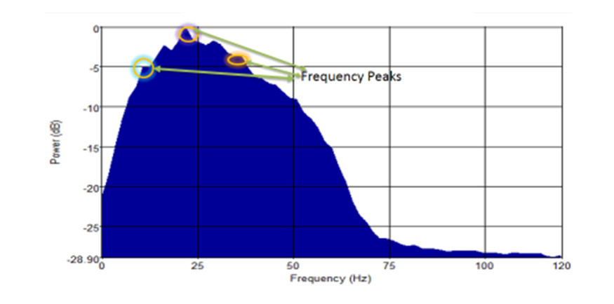
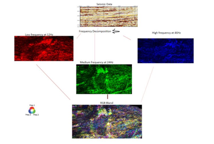
From the amplitude spectrum generated, the individual spectral components at different frequencies of the horizon [low (12 Hz), medium (24 Hz), and the highest frequency (46 Hz)] are selected (Figure 9). Longer wavelengths with low frequencies (red) are absorbed in a shallow depth while shorter wavelengths (blue) penetrates to a deeper depth. Therefore, higher frequencies with short wavelengths (blue) can penetrate deeper. The higher the frequency, the thinner the bed and vice versa. The highest of these frequencies (the dominant peak frequency) is selected.

White spectrum is produced in which all frequencies contribute to the power. The frequency decreases with depth because of attenuation and when the frequency is low, it images thicker beds. The low frequency at shallow depth is indicative of thicker beds while high frequency as we go deeper indicates thin beds. Individual spectral decomposition frequency slices (at single frequencies of 12 Hz, 24 Hz and 46 Hz) or volumes are displayed with different colour schemes for Horizons 1 and 2. There are different colour options used which represent low, medium and high frequencies at varying depth. These are combined to blend multiple spectrally decomposed images. The one used in this research was Red-Green-Blue (RGB). With RGB, the three discrete frequencies were selected and plotted against red, green, and blue. The frequency at 12 Hz showed the thickest part of the channel at shallow depth, the frequency at 24 Hz shows the thicker part of the channel while 46 Hz illuminates the thinnest part of the channel i.e. the higher the frequency, the thinner the bed.
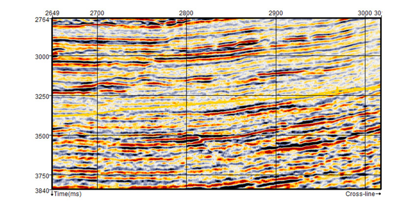
From the input field data, some traces were missing while some reflections have been lost to the chaotic high depositional energy/trend with truncations of seismic events and amplitude changes along with seismic events (Figure 10a). Parts of the sections with chaotic reflections suggests either relatively high depositional energy, the variability of conditions during deposition, or disruption after deposition. High frequency and thin geometry of deltaic channels were observed after spectral decomposition. Figure 10b showed the seismic data regularization section. Here, all traces are seen with the continuity of reflections. Comparing this result to the input data, it showed that the continuity of the seismic reflections is much improved. Other geologic structures are also revealed.

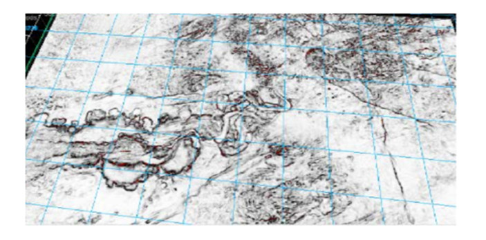
Due to poor resolution of the data and complexity of the geology, seismic attributes such as trace, variance etc. were used to enhance the structures observed in the section. Complex and meandering channels, as well as lobes, are observed at the centre of the field using variance attribute (Figure 11). The channels appear to be regional as it extends through the section. It provided a better idea of the channel continuity and possible reservoir quality. These are likely traps for hydrocarbon.

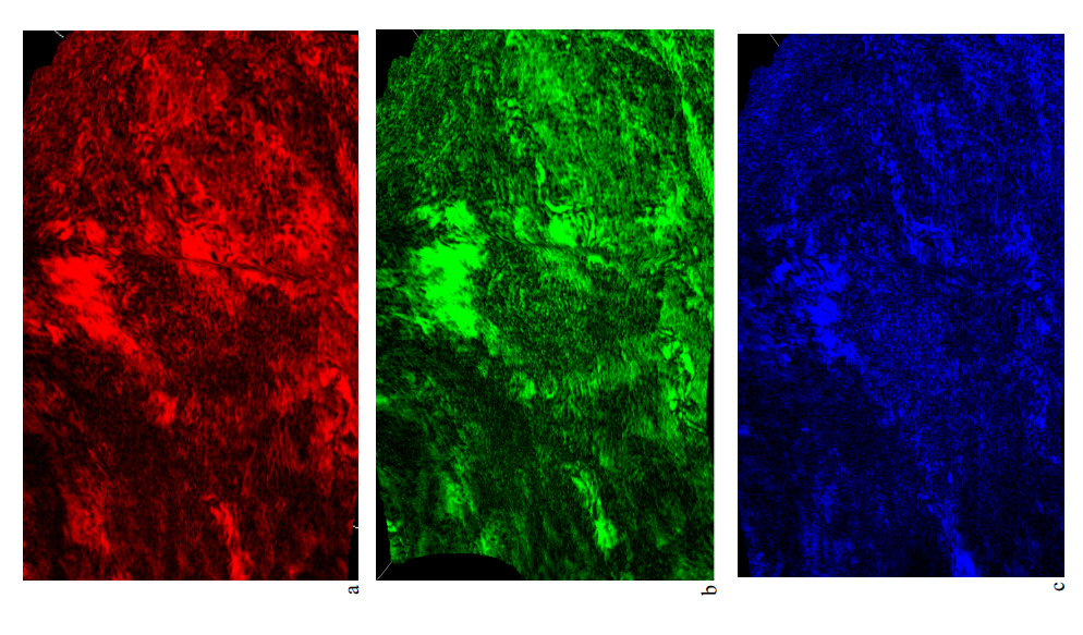
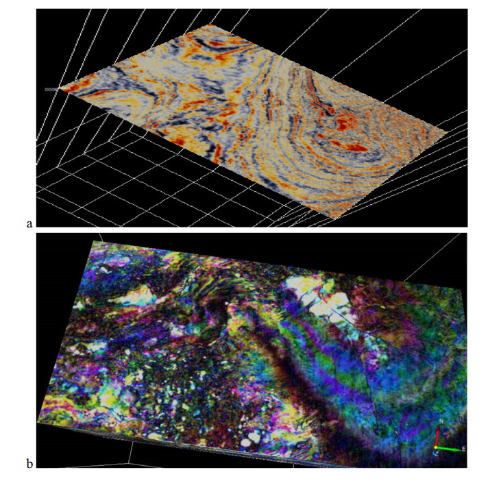
Two horizons (Horizons 1 and 2) were mapped based on the continuity of the reflections on the seismic section. The spectra was used to delineate the stratigraphy (lithology) and thin-bed thickness variability. Large and detailed shapes are easily detected than small or blurry shapes i.e. short and low frequency but when the frequency is enhanced, the vertical resolution improves and subtle geologic features are revealed. Geologic discontinuities are easily identified through the phase spectra while channel sands and subtle fault systems were delineated from the Stratigraphic setting. Individual frequency slices were generated from the interpreted horizons. Figure 12a-c illustrates spectral decomposition slices for horizon 1 at different frequencies of 12 Hz, 24 Hz and 46 Hz.

The data is decomposed into multiple bands of different frequencies which revealed different parts of the information. Changes can be observed from the three frequency responses at 12 Hz, 24 Hz and 46 Hz which showed subtle differences. Viewing the frequency responses individually and also comparing them showed how the energy is changing. Running a frequency decomposition centred around 12 Hz, we get the 12 Hz response (a localised response). It revealed a narrow bandwidth data response i.e. a part of the frequency spectrum with poor vertical resolution and smearing. The discreet layers cannot be identified accurately. It’s hard to define the top and the base of the horizon. It’s much easier combining them into one volume through the RGB blend. The 12 Hz frequency response represents the red channel, 24 Hz response is the green channel while the 46 Hz response is the blue channel. This gives a blend of the contribution to produce the RGB volume. The workflow of the spectral decomposition is illustrated in Figure 13.

Figure 14 illustrates Red-Green-Blue blend of the higher resolution of the three frequency slices for horizon 1 at depth. The RGB colour blend effect gives a better understanding of the geology of deep-water sedimentary and enhances exploitation benefits within the thin reservoirs. The colour blend is spectral balancing which recompense for wavelet and energy loss. The figure showed a complex meandering river system and other less winding channels which are discontinuous and difficult to resolve on the seismic. The magnitude response of the frequency which is high within the thin beds made it easy to interpret the stratigraphy. The RGB colour blending slices revealed more hidden structures compared with what is observed in the time structural map. This gives more confidence in mapping and interpretation. When the colour is white, it means there is high amplitude response in all the three volumes; where there is black, it showed low amplitude response of the three volumes and when one colour is dominating, it showed that the frequency is dominating at that point. It revealed the geometry of the channels and other fewer sinusoidal channels. Towards the northern part of the system, the bed thins. The amplitude response decreases and it is dominated by blue colour which is high frequency. At the central part, there is high amplitude, an indication of hydrocarbon/gas effect. The acoustic impedance within the gas-bearing sand is lower compared to the surrounding shale [26]. At the lower part where there’s a change in colour to brownish, it showed thickening up of the reflectors and greater contribution from the lower frequencies. There are changes in colour in the channel system which could be indicative of changes in lithology. The Frequency decomposition and RGB blend are applicable at all stages, from exploration, appraisal, development and production. The channels are displayed with bright colouration which contains multiple frequencies. Major channel discontinuity was also observed within the low frequency. The meandering channels run across from the north-eastern to the south-western part. These are likely traps for hydrocarbon accumulation [17].

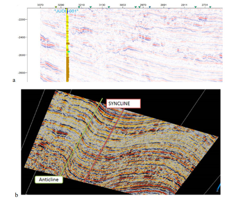
A major geologic feature was observed on the time-slice from the divergent pattern on the seismic section as we penetrate deeper, which is an Unconformity (Figure 15a, b). This represents a significant break in vertical velocity or breaks in deposition time or record on Horizon [27]. The concept of unconformity was presented as part of the rock cycle by [28,29]. This type of unconformity is called Angular Unconformity [30,31,32]. Angular Unconformity is an unconformity between two groups of rocks whose bedding planes are not parallel or in which the older underlying rock dips at a different angle (usually steeper) than the younger, overlying strata. Its interpretation depends on the recognition of characteristic reflection geometries rather than on amplitude information. It shows that deposition of the sediments took place at different times. This is further confirmed from the seismic section in Figure 16.


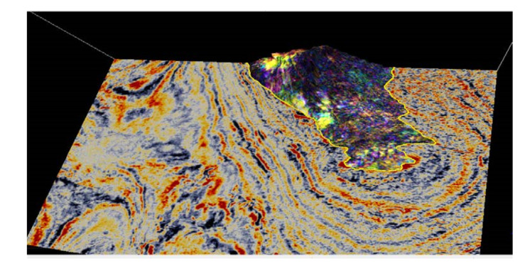
From the time-slice, a huge northwest-southeast trending detached anticlinal fold is also observed in the north-eastern part of the field (Figure 17). This could be as a result of differential loading on the ductile marine Akata shale that is under-compacted and over-pressured as well as the gravitational collapse of the continental slope from an influx of sediments [33]. Associated with these structures are the dominant hydrocarbon traps in the Niger Delta which are suggested probable zone or new drilling site. The horizons fall within the anticlinal fold which is a structural trap.

From the amplitude spectral, the high amplitude is direct hydrocarbon indicators of the presence of hydrocarbon within the reservoirs.
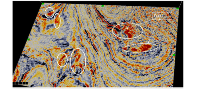
Finally, structural highs extend within the field in the north-eastern direction which is a probable location for drilling new wells of economic quantity. There is an anomaly observed at the north-eastern Part and the western part of the field (Figure 18). It is high amplitude which is indicative of a bright spot. This is as a result of a change in pore fluid. The portion of the field is where the thin beds are. It means that the anomaly is caused by the gas effect. This is very important in hydrocarbon exploration wells.

The south-western part of the field is structurally lows. Integrating the information from geological constraints, seismic data and spectral decomposition parameters has improved the resolution and provided direct attributes for stratigraphic interpretation. Thus, it ascertained the reservoirs within portions of interest.
Limited bandwidth and poor vertical resolution make it difficult when using conventional seismic interpretation to detect or resolve the geology within a complex zone. Therefore, spectral decomposition has been used effectively to image and map structural and stratigraphy changes showing subtle geologic features of great importance within the Petroleum system for hydrocarbon accumulation.
This research work has shown the importance of Spectral Decomposition method for reservoir characterisation especially in complex by-passed areas with subtle geologic features. Despite the limited vertical resolution of the seismic, Spectral Decomposition was used for effective stratigraphic and structural delineation in “Jude Field”, Offshore Niger Delta, Nigeria. Erroneous appraisal of seismic amplitude may lead to inaccurate interpretation and increase exploration risks. The result showed the validity of the technique and was also used to propose a new drilling site. Modern exploration technology with enhanced oil recovery techniques can be successfully adopted to harness the hydrocarbon in these by-passed zones where drilling was once uneconomic. This will further lead to an increase the productivity within the field and development in the national revenue.
The authors express their thanks to TWAS/CNPq for funding the research. Special thanks to the Federal University of Technology, Akure, Ondo State, Nigeria and Institute of Energy and Environment, University of Sao Paulo, Sao Paulo, Brazil for the opportunity to carry out the project. Final appreciation to the Shell Nigeria Exploration and Production Company Limited (SNEPCo) for the data used for the research.
All authors declare no conflicts of interest in this paper.
| [1] |
Partyka G, Gridley J, Lopez J (1999) Interpretational applications of spectral decomposition in reservoir characterization. Lead Edge 18: 353-360. doi: 10.1190/1.1438295

|
| [2] |
Marfurt KJ, Kirlin RL (2001) Narrow-band spectral analysis and thin-bed tuning. Geophysics 66: 1274-1283. doi: 10.1190/1.1487075
|
| [3] |
Castagna JP, Sun S, Siegfried RW (2003) Instantaneous spectral analysis; Detection of low-frequency shadows associated with hydrocarbons. Lead Edge 22: 120-127. doi: 10.1190/1.1559038
|
| [4] |
Sinha S, Routh PS, Anno PD, et al. (2005) Spectral Decomposition of Seismic Data with continuous wavelet transform. Geophysics 70: 19-25. doi: 10.1190/1.2127113
|
| [5] |
Tomasso M, Bouroullec R, Pyles DR (2010) The use of spectral recomposition in tailored forward seismic modelling of outcrop analogs. AAPG Bull 94: 457-474. doi: 10.1306/08240909051
|
| [6] | Telford WM, Geldart LP, Sheriff RE (1971) Applied Geophysics, Second Edition, 1-270. |
| [7] |
Taner MT, Koehler F, Sheriff RE (1979) Complex seismic trace analysis. Geophysics 44: 1041-1063. doi: 10.1190/1.1440994
|
| [8] |
Latimer RB, Davison R, Van Riel P (2000) An Interpreter's guide to understanding and working with seismic-derived acoustic impedance data. Lead Edge 19: 242-256. doi: 10.1190/1.1438580
|
| [9] |
Abdel-Fattah M, Gameel M, Awad S, et al. (2015) Seismic interpretation of the Aptian Alamein Dolomite in the Razzak Oil field, Western Desert, Egypt. Arabian J Geosci 8: 4669-4684. doi: 10.1007/s12517-014-1595-4
|
| [10] |
Fadul MF, El Dawi MG, Abdel-Fattah MI (2020) Seismic interpretation and the tectonic regime of Sudanese Rift System: Implications for hydrocarbon exploration in neem field (Muglad Basin). J Pet Sci Eng 2020: 107223. doi: 10.1016/j.petrol.2020.107223
|
| [11] | Sheriff RE (2002) Encyclopaedic Dictionary of Applied Geophysics, Fourth Edition, Society of exploration geophysicists. |
| [12] | Cohen L (1995) Time Frequency Analysis, Prentice Hall, New Jersey. |
| [13] | Castagna JP, Sun S (2006) Comparison of Spectral Decomposition methods. First Break 24: 3-24. |
| [14] |
Chakraborty A, Okaya D (1995) Frequency-time Decomposition of seismic data suing wavelet based. Geophysics 60: 1906-1916. doi: 10.1190/1.1443922
|
| [15] | Weber KJ, Dakouru E (1975) Petroleum Geology of the Niger Delta. Proceedings of the Ninth World Petroleum Congress. Geology: London, Applied Science Publishers, Ltd, 2: 210-221. |
| [16] | Burke K (1972) Long-shore drift, submarine canyons, and submarine fans in development of Niger Delta: AAPG Bull 56: 1975-1983. |
| [17] | Doust H, Omatsola E (1990) Niger Delta, Divergent/Passive margin basins. AAPG Bull, 239-248. |
| [18] | Short KC, Stauble AJ (1967) Outline of Geology of Niger Delta. AAPG Bull 51: 761-779. |
| [19] | Avbovbo AA (1978) Tertiary litho-stratigraphy of Niger Delta. AAPG Bull 62: 295-300. |
| [20] | Kulke H (1995) Regional Petroleum Geology of the World. Part Ⅱ: Africa, America, Australia and Antarctica. Berlin, Gebrüder Borntraeger, 143-172. |
| [21] | SPDC (2005) Supply Chain Management Practice, Shell Petroleum Development Limited, Nigeria. Available from: http://www.ipsa.co.za/bola%20afolabi.ppt. |
| [22] |
Abraham-A RM, Taoili F (2018) Hydrocarbon Viability Prediction of Some Selected Reservoirs in Osland Oil and Gas Field, Offshore Niger Delta, Nigeria. Mar Pet Geol 100: 195-203. doi: 10.1016/j.marpetgeo.2018.11.007
|
| [23] |
Pigott JD, Kang MH, Han HC (2013) First Order Seismic Attributes for clastic Seismic facies Interpretation: Examples from the East China Sea. J Asian Earth Sci 66: 34-54. doi: 10.1016/j.jseaes.2012.11.043
|
| [24] | Widess M (1973) How Thin is a Thin Bed? Geophysics 38: 1176-1180. |
| [25] |
Zhu Y, Huang C (2012) An Improved Median Filtering Algorithm for Image Noise Reduction. Phys Procedia 25: 609-616. doi: 10.1016/j.phpro.2012.03.133
|
| [26] |
Naseer MT, Asim S (2017) Detection of cretaceous incised valley shale for resource play, Miano gas field, SW Pakistan: Spectral Decomposition using continuous wavelet transform. J Asian Earth Sci 147: 358-377. doi: 10.1016/j.jseaes.2017.07.031
|
| [27] | Neuendorf KKE, Mehl JP, Jackson JA (2005) Glossary of Geology, Fifth Edition. American Geological Institute, Alexandria, Virginia, 779. |
| [28] | Hutton J (1788) Theory of the Earth; or An Investigation of the Laws Observable in the Composition, Dissolution, and Restoration of Land upon the Globe. Earth and Environmental Science Transactions of the Royal Society of Edinburgh, 1: 209-304. |
| [29] | Hutton J (1795) Theory of the Earth with Proofs and Illustrations. (Edinburgh)/London: Geological Society, I and Ⅱ: 1795-1899. |
| [30] | Jameson R (1805) A mineralogical description of the County of Dumfries. Bell & Bradfute, 1-75. |
| [31] | De la Beche HT (1830) Sections and Views Illustrative of Geological Phenomena. Treuttel & Wurtz, Cambridge University Press, London, 177. |
| [32] | Lyell C, Deshayes GP (1830) Principles of geology: being an attempt to explain the former changes of the earth's surface, by reference to causes now in operation. J. Murray, 511. |
| [33] | Uko ED, Emudianughe JE, Tamunobereton-ari I (2013) Page Overpressure Prediction in the North-West Niger Delta, using Porosity Data. J Appl Geol Geophys 1: 42-50. |
| 1. | Oyelowo Gabriel Bayowa, Theophilus Aanuoluwa Adagunodo, Adeola Opeyemi Oshonaiye, Bisola Stella Boluwade, Mapping of thin sandstone reservoirs in bisol field, Niger delta, Nigeria using spectral decomposition technique, 2021, 12, 16749847, 54, 10.1016/j.geog.2020.11.002 | |
| 2. | Mohammed S. Gumati, Seismic evidence for the syndepositional fault activity controls on geometry and facies distribution patterns of Cenomanian (Lidam) reservoir, Dahra Platform, Sirt Basin, Libya, 2022, 136, 02648172, 105471, 10.1016/j.marpetgeo.2021.105471 | |
| 3. | Anthony I Nzekwu, Richardson M Abraham-A, Reservoir sands characterisation involving capacity prediction in NZ oil and gas field, offshore Niger Delta, Nigeria, 2022, 8, 2471-2132, 159, 10.3934/geosci.2022010 | |
| 4. | Richardson M. Abraham-A, Fabio Taioli, Anthony I. Nzekwu, Physical properties of sandstone reservoirs: Implication for fluid mobility, 2022, 3, 26667592, 349, 10.1016/j.engeos.2022.06.001 | |
| 5. | Oluwatoyin Abosede Oluwadare, Adetayo Femi Folorunso, Olusola Raheemat Ashiru, Stephanie Imabong Otoabasi-Akpan, High resolution 3-D seismic and sequence stratigraphy for reservoir prediction in ‘Stephi’ field, offshore Niger Delta, Nigeria, 2024, 14, 2045-2322, 10.1038/s41598-024-73285-z | |
| 6. | Aslıhan Nasıf, Enhancing low- and high-frequency components of the seismic data to emphasise BSRs and bright spots and implications for seismic attribute analysis, 2024, 133, 0973-774X, 10.1007/s12040-023-02241-8 | |
| 7. | M.A. Bello, M.I. Oladapo, M.R. Abraham-A, O.M. Orji, Aquifer integrity test using the Dar Zarouk parameters in Emure Ekiti Southwestern Nigeria, 2025, 3, 22117148, 100087, 10.1016/j.rines.2025.100087 | |
| 8. | O.A. Oluwadare, P.A. Enikanselu, F. Taoili, M.T. Olowokere, Thin-Compartmented Reservoir Simulation and Quantitative Interpretation Using Seismic Attributes: A Case Study in ‘Jude Field’, Offshore Niger Delta, 2025, 3, 2786-9342, 343, 10.59324/ejaset.2025.3(3).24 |
O. A. Oluwadare, M.T. Olowokere, F. Taoili, P.A. Enikanselu, R.M. Abraham-Adejumo. Application of time-frequency decomposition and seismic attributes for stratigraphic interpretation of thin reservoirs in "Jude Field", Offshore Niger Delta[J]. AIMS Geosciences, 2020, 6(3): 378-396. doi: 10.3934/geosci.2020021

 DownLoad: