A nonparametric copula distribution framework for bivariate joint distribution analysis of flood characteristics for the Kelantan River basin in Malaysia

1.   Introduction

The Kelantan River basin in Malaysia is often subjecting to most severe monsoonal flooding and perceiving for increasing in term of their frequency and magnitude ^[1,2,3]. The expectation of the occurrence of catastrophic flooding has increased from once in every 50 years to 15 years from 2004 in the Kelantan region ^[1,3,4]. For example, the intense and prolonged precipitation in the year 2002 caused flooding of a total area of 1640 km² and affected the total of about 714,287 people or in the year December 2014, much heavy precipitation triggered the flood event in the several parts of the east coast of the Kelantan river basin and affected more than 200,000 people ^[3]. Hussain and Ismail (i.e., ^[5]), study revealed that the Gulliemard Bridge, Lebir and Galas gauge stations have highest in the flood frequency rather than Nenggiri station. Similarly, Nashwan et al. (i.e., ^[6]) literature pointed that the downstream area of this river basin is the highest risk of devastating flood events. The cause of frequent failure of hydrologic or flood defence infrastructure in Malaysia due to the impact of moderately severe of flood episodes might be attributed due to the lack of complete flood hydrograph or in other words, where only flood peak discharge samples often targeted in deriving the flood frequency curve during the structural development.

Flood is a multidimensional stochastic consequence usually characterized completely through its trivariate interdependence vectors i.e., flood peak flow, volume and duration of flood hydrograph ^[7,8]. Flood frequency analysis (FFA) is an approach of establishing the relationship between flood design quantiles and their frequency of occurrence or non-exceedance probabilities by fitting probability distribution functions (PDFs) ^[9]. Earlier efforts frequently incorporated the univariate FFA (i.e., ^[10]) but the necessity of estimating flood design hydrograph instead of design quantiles derived from single variable flood episodes motivated numerous literatures towards the joint probability analysis of flood characteristics using different traditional multivariate functions i.e., Krstanovic and Singh ^[11], Yue ^[12] and Escalante and Raynal ^[13]. Such distribution-based modelling approaches often surrounded with several statistical constraints and limitations such as, (1) each flood vectors must assume to have normal distributions or either transformed to have normal distributions; (2) if the number of variables are increased then mathematical formulation becomes more complex and complicated; (3) statistical parameter of univariate marginal structure is often employed to model their joint dependence structure; (4) limited space are available to justify joint dependence structure etc, ^[7,8,14]. Hence to over the above challenges, De Michele and Salvadori (i.e., ^[15]), firstly incorporated copulas for establishing the joint dependence structure between storm intensity and duration. The copulas function segregated the modelling of individual univariate vectors and their joint structure separately into two distinct stages, thus attributed higher flexibility in the selection of best-fitted marginal distributions not necessary from the same family of probability distributions and also their joint structure to capture a wider extent of mutual concurrency and also, preservation in their joint association ^[16,17]. Numerous literatures incorporated bivariate or few trivariate copulas distribution as a model risk for tackling different hydrological extremes issues such as, flood modelling ^[18,19], drought modelling ^[14] rainfall or storm modelling ^[20] or either modelling of hydro-climatic extremes ^[21] etc.

The multivariate FFA either with or without copulas has been applied frequently with parametric distributions where the parametric functions are often employed to modelled univariate marginal distributions and the parametric copulas function for establishing their joint dependence structure. But, the parametric functions always imposed an assumption that the random samples are coming from the known populations whose PDF are pre-defined i.e., the marginal distribution is assumed to follow some specific family of parametric functions ^[22]. In actual, no universal rules and studies are imposed to model any hydrologic vectors through any fixed or pre-defined distribution functions, which would follow different distributions and desire to model separately or in other words, the best-fitted marginal distributions not be from the same probability distribution family ^{[23,24,25,26]}. Also, according to Dooge ^[27], it is already pointed out that no amount of statistical refinement can overcome the consequences due to lack of prior distribution information of the observed random samples also, it would be quite difficult to approximate distribution tail beyond largest values under the parametric framework ^[28]. Therefore, in the past few decades, an attempt via kernel density estimators or KDE recognized as a much flexible and stable non-parametric data smoothing procedure to inference about the populations based on the finite observational samples and thus motivated in the field of hydrologic or flood frequency analysis and which often yielding a bonafide density function ^{[22,23,29,30]}. Nonparametric framework didn't require any prior distribution assumptions and will be directly retrieved from distributed series with a higher extent of flexibility in their univariate function as compared with parametric density estimators ^[23,31]. From the above review, it is also conclude that few work already performed the univariate nonparametric FFA i.e., Adamowski (i.e., ^[23]), Lall (i.e., ^[32]), but only limited literature focused over the establishment of copula-based methodologies under nonparametric or semiparametric framework i.e., Karmakar and Siminovic ^[22,33] and Reddy and Ganguli ^[9], performed bivariate flood modelling using a mixed marginal distribution from the parametric and nonparametric families of probability distributions. In both cases, the parametric copulas are employed to modelled the joint distribution of flood characteristics. On other side, the Chen and Huang (i.e., ^[34]) study demonstrated a bivariate kernel copula framework for handling the problem of boundary bias. Actually, if the targeted copulas and univariate marginal distributions belongs to some specific parametric families, it might be problematic, if the underlying assumption are violated. Therefore, these nonparametric distribution framework can ameliorate these modelling issues and can be able to produce a significant outcomes without assuming a particular form for the univariate marginal or multivariate copula distributions.

A study performed by Shahid and Firuza (i.e., ^[35]) over this river basin already demonstrated the modelling of trivariate joint distribution of flood characteristics by introducing the 3-D copula functions under the parametric settings and also pointed the importance of trivariate joint and conditional return periods. This literature introduced the concept and importance of nonparametric copula-based methodology in the establishment of multivariate FFA. In this study we demonstrated the efficacy of nonparametric copula distribution where both parametric and nonparametric marginal distribution functions are separately conjoined by a nonparametric copulas framework and applied as case study for the daily basis streamflow discharge records from period 1961–2016 for the Kelantan River Basin at the Gulliemard Bridge gauge station in Malaysia. This study pointed two different modelling approach for estimating the bivariate joint dependency. The first simulation approach comprises the modelling of nonparametric marginal distribution with a nonparametric copulas and the second approach consisting the modelling of parametric marginal distribution with a nonparametric copula.

2.   Study area

The Gulliemard bridge station is located at the downstream of Kelantan river near the Kuala Kari region. The geographical location of this river basin is Lat 4°30′ N to 6°15′ N and Long 101°E to 102°45′ E. It is the longest river of Kelantan state, which originating from the Tahan mountain range to the South China Sea in the north-eastern part of Peninsular Malaysia. The river is about 248 km long with a drain area of 13,100 km² and which occupying more than 85% of the state of Kelantan. The estimated runoff is about 500 m³sec⁻¹ and the variations of annual precipitations for this region in between 0 mm (dry period)–1750 mm (wet or north-eastern monsoonal period) (i.e., ^[1]). The major land use of this area is agriculture (i.e., paddy, rubber and oil palm) for midstream and downstream and forest for upstream (i.e. near to Gua Musang). Few studies over this region such as Chan ^[4], Adnan and Atkinson ^[3], pointed that such extreme hydrologic consequences are mainly due to rapid human intervention from natural to land use activities in the form of deforestations or land clearance either for promoting the agricultural activities through palm oil and rubber plantations or either due to logging activities.

3.   Proposed methodology and data analysis

3.1.   Delineation of trivariate flood characteristics

Annual (Maximum) series or AM also called block (annual) maxima and Peak over Threshold (or POT) are the two holistic technique widely accepted in the extreme probability simulations ^[36]. In this study we adopted the AM approach to extract the trivariate flood characteristics. Figure 1, illustrates a typical flood hydrograph showing the delineation of trivariate flood characteristics. The flood peak flow, P, values are estimated using the maximum streamflow discharge records at an annual scale using Eq 1, which indicated that for each year there is only one flood episodes at the targeted site (refer to Figure 1) ^[9,37]. Referred to same Figure 1, the flood duration (D) samples are estimated by recognizing the time of rise and fall of the flood hydrograph (i.e., points at Q_is and Q_ie in the Figure 1) and volume (V) samples are obtained using Eqs 2 and 3 (i.e., ^[9,37]).

Figure 1.  A typical hydrograph showing flood characteristic (Source: Adapted from Latif and Mustafa ^[35]).

DownLoad: Full-Size Img PowerPoint

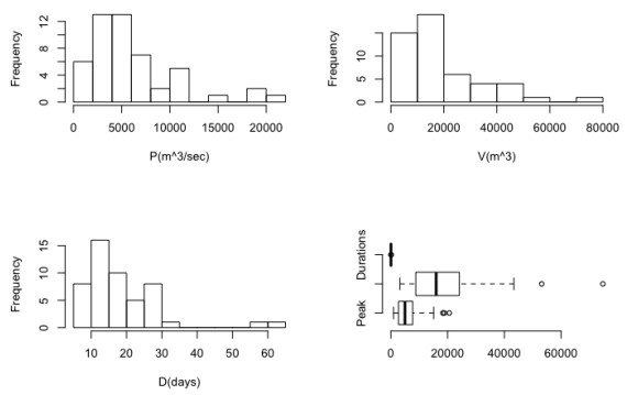
where ${{\rm{Q}}_{{\rm{ij}}}} =$ j^th days streamflow magnitude for the i^th year; ${{\rm{Q}}_{{\rm{is}}}}{\rm{\;and\;}}{{\rm{Q}}_{{\rm{ie}}}} =$ streamflow magnitude for the start date ${\rm{S}}{{\rm{D}}_{\rm{i}}}$ and end date ${\rm{E}}{{\rm{D}}_{\rm{i}}}{\rm{}}$ of the flood runoff. The descriptive statistics of the derived flood characteristics are listed in Table 1 and their visual interpretations, via the histogram plot and box-whisker plot are illustrated in the Figure 2.

Table 1.  Descriptive statistics of flood characteristics.

Descriptive statistics	P (m3/sec)	V (m3)	D (days)
Sample Size	50	50	50
Range	19670	71558	57
Mean	6078	19122	19.04
Variance	2.15E+07	2.14E+08	117.75
Std. Deviation	4639	14623	10.851
Coef. of Variation	0.76324	0.76473	0.56993
Skewness (Pearson)	1.506	1.590	2.210
Kurtosis (Pearson)	1.883	2.864	6.252
Min	916.3	3182.3	7
25% (Q1)	2671.8	8668.5	12
50% (Median)	4961	15959	16
75% (Q3)	7711.7	24476	25
Max	20586	74740	64

---

 | Show Table

DownLoad: CSV

Figure 2.  Visualizing the annual flood characteristics using the histogram distribution and Box-whisker plot.

DownLoad: Full-Size Img PowerPoint

3.2.   Univariate analysis

3.2.1.   Parametric marginal distribution analysis

In this study, we introduced both the set of parametric and nonparametric distributions for characterizing the flood marginals. Several models often would fit the data equally well but, each would give different estimates of a given quantile especially in the tails of distribution ^[22]. A distinguish varieties of parametric functions are tested as a possible marginal distribution, referred to Table 2. The parameters of each fitted distributions are estimated using the maximum likelihood estimation (MLE) (i.e., ^[38]), method of moments (MOM) (i.e., ^[38]), least square method (LS), and L statistics-based method of L-moments (i.e., ^[36]). All the univariate fitting procedure are carried out using the Easyfit software (Mathwave Technologies 2004–2017). After that, the best-fitted distributions are selected for each individual flood characteristics using the different goodness-of-fit test statistics.

Table 2.  The mathematical expressions for probability density functions (PDF) of different parametric families functions.

Parametric functions	Probability density function (or PDF)	Remarks
Gamma (2P) & (3P)	${\rm{f}}\left({\rm{x}} \right) = {\rm{}}\frac{{{{\left({{\rm{x}} - {\rm{ \mathsf{ γ} }}} \right)}^{{\rm{ \mathsf{ α} }} - 1}}}}{{{{\rm{ \mathsf{ β} }}^{\rm{ \mathsf{ α} }}}{\rm{\Gamma }}\left({\rm{ \mathsf{ α} }} \right)}}{{\rm{e}}^{\frac{{ - \left({{\rm{x}} - {\rm{ \mathsf{ γ} }}} \right)}}{{\rm{ \mathsf{ β} }}}}}{\rm{}}\& f\left({\rm{x}} \right) = {\rm{}}\frac{{{{\rm{x}}^{{\rm{ \mathsf{ α} }} - 1}}}}{{{{\rm{ \mathsf{ β} }}^{\rm{ \mathsf{ α} }}}{\rm{\Gamma }}\left({\rm{ \mathsf{ α} }} \right)}}{{\rm{e}}^{\frac{{ - {\rm{x}}}}{{\rm{ \mathsf{ β} }}}}}{\rm{}}$	${\rm{ \mathsf{ α} }} > 0, \beta > 0, \gamma > 0$- shape, scale and locations parameter; ${\rm{ \mathsf{ γ} }} \equiv 0{\rm{}}$ yield 2-parameter gamma structure
GEV(3P)	${\rm{f}}\left({\rm{x}} \right) = \frac{1}{{\rm{ \mathsf{ σ} }}}{{\rm{e}}^{ - {{\left({1 + {\rm{kz}}} \right)}^{ - 1/{\rm{k}}}}{{\left({1 + {\rm{kz}}} \right)}^{ - 1 - 1/{\rm{k\;\;\;}}}}}}{\rm{for\;k}}\; \ne 0{\rm{}}$ $\frac{1}{{\rm{ \mathsf{ σ} }}}{{\rm{e}}^{\left({ - 1 - {{\rm{e}}^{\left({ - {\rm{z}}} \right)}}} \right)}}{\rm{\;for\;k}} = 0$	${\rm{k}}\left({{\rm{shape}}} \right), {\rm{ \mathsf{ σ} }}\left({{\rm{scale}}} \right), {\rm{ \mathsf{ μ} }}\left({{\rm{location}}} \right)$, such that, ${\rm{ \mathsf{ σ} }} > 0$ & ${\rm{z}} \equiv \left({\left({{\rm{x}} - {\rm{ \mathsf{ μ} }}} \right)} \right)/{\rm{ \mathsf{ σ} }}$ Domain: $1 + {\rm{k}}\left({{\rm{x}} - {\rm{ \mathsf{ μ} }}} \right)/{\rm{ \mathsf{ σ} \; for\; k}} \ne 0{\rm{}}\& - \infty < x < + \infty \; for\; k = 0$
Inv. Gaussian (2P)	${\rm{f}}\left({\rm{x}} \right) = \sqrt {\frac{{\rm{ \mathsf{ λ} }}}{{2{\rm{ \mathsf{ π} }}{{\rm{x}}^3}}}} {{\rm{e}}^{ - \frac{{{\rm{ \mathsf{ λ} }}{{\left({{\rm{x}} - {\rm{ \mathsf{ μ} }}} \right)}^2}}}{{2{{\rm{ \mathsf{ μ} }}^2}\left({\rm{x}} \right)}}}}{\rm{}}$	${\rm{ \mathsf{ λ} }} > 0, \mu > 0(continuous\; parameter, {\rm{ \mathsf{ γ} }}\left({{\rm{location}}\; {\rm{parameter}}} \right){\rm{}}$ for ${\rm{ \mathsf{ γ} }} < x < + \infty$
Johnson SB(4P)	${\rm{f}}\left({\rm{x}} \right) = {\rm{}}\frac{{\rm{ \mathsf{ δ} }}}{{{\rm{ \mathsf{ λ} }}\sqrt {2{\rm{ \mathsf{ π} }}} {\rm{z}}\left({1 - {\rm{z}}} \right)}}{{\rm{e}}^{ - 0.5{{\left({{\rm{ \mathsf{ γ} }} + {\rm{ \mathsf{ δ} }}\ln \frac{{\rm{z}}}{{1 - {\rm{z}}}}} \right)}^2}}}$	Domain: ${\rm{ \mathsf{ ξ} }} \le {\rm{x}} \le {\rm{ \mathsf{ ξ} }} + {\rm{ \mathsf{ λ} }}$ ${\rm{ \mathsf{ γ} }}, {\rm{ \mathsf{ δ} }} > 0\left({{\rm{shape}}} \right); {\rm{ \mathsf{ λ} }} > 0\left({{\rm{scale}}} \right); {\rm{ \mathsf{ ξ}\; location}}\; {\rm{parameter}})$
Log-Gamma (2P)	${\rm{f}}\left({\rm{x}} \right) = \frac{{{{\left({\ln {\rm{x}}} \right)}^{{\rm{ \mathsf{ α} }} - 1}}}}{{{\rm{x}}{{\rm{ \mathsf{ β} }}^{\rm{ \mathsf{ α} }}}{\rm{\Gamma }}\left({\rm{ \mathsf{ α} }} \right)}}{{\rm{e}}^{ - \left({\frac{{\ln {\rm{x}}}}{{\rm{ \mathsf{ β} }}}} \right)}}$	Domain: $0 < x < + \infty$ ${\rm{ \mathsf{ α} }} > 0, \beta > 0\left({shape\; parameter} \right)$
Log-Logistic (2P)	${\rm{f}}\left({\rm{x}} \right) = {\rm{}}\frac{{\rm{ \mathsf{ α} }}}{{\rm{ \mathsf{ β} }}}{\left({\frac{{\rm{x}}}{{\rm{ \mathsf{ β} }}}} \right)^{{\rm{ \mathsf{ α} }} - 1}}{\left({1 + {{\left({\frac{{\rm{x}}}{{\rm{ \mathsf{ β} }}}} \right)}^{\rm{ \mathsf{ α} }}}} \right)^{ - 2}}$	Domain: ${\rm{ \mathsf{ γ} }} < x < + \infty$ ${\rm{ \mathsf{ α} }} > 0\left({{\rm{shape}}} \right); {\rm{ \mathsf{ β} }} > 0\left({{\rm{scale}}} \right)$
Lognormal (2P)	${\rm{f}}\left({\rm{x}} \right) = {\rm{}}\frac{{{{\rm{e}}^{ - 0.5{{\left({\frac{{\ln \left({\rm{x}} \right) - {\rm{ \mathsf{ μ} }}}}{{\rm{ \mathsf{ σ} }}}} \right)}^2}}}}}{{\left({\rm{x}} \right){\rm{ \mathsf{ σ} }}\sqrt {2{\rm{ \mathsf{ π} }}} }}{\rm{}}$	${\rm{ \mathsf{ σ} }} > 0\left({{\rm{shape}}\; {\rm{parameter}}} \right);$ ${\rm{ \mathsf{ μ} }}\left({{\rm{scale}}\; {\rm{parameter}}} \right)$
Weibull (2P)	${\rm{f}}\left({\rm{x}} \right) = {\rm{}}\frac{{\rm{ \mathsf{ α} }}}{{\rm{ \mathsf{ β} }}}{\left({\frac{{\rm{x}}}{{\rm{ \mathsf{ β} }}}} \right)^{{\rm{ \mathsf{ α} }} - 1}}{{\rm{e}}^{ - {{\left({\frac{{\rm{x}}}{{\rm{ \mathsf{ β} }}}} \right)}^{\rm{ \mathsf{ α} }}}}}$	Domain: ${\rm{ \mathsf{ α} }} > 0\left({{\rm{shape}}} \right), {\rm{ \mathsf{ β} }} > 0\left({{\rm{scale}}} \right){\rm{}}$

---

 | Show Table

DownLoad: CSV

The parametric functions always imposed an assumption that the random samples are coming from the known populations whose PDF are pre-defined (see section 1). In other words, the marginal distribution of flood characteristics is assumed to follow some specific family of parametric density functions ^[22]. But in actual, no universal rules and studies are imposed to model any hydrologic vectors through any fixed or pre-defined distribution functions, which would follow different distributions and desire to model separately. Therefore, analysis based on the parametric concept would might reveal for uncertainty in the estimated design quantiles because the parametric distributions do not always represent the characteristics of the data, appropriately.

3.2.2.   Nonparametric estimates of flood marginal distributions

The concept and idea of kernel density estimators or KDE are firstly introduced by the Rosenblatt ^[39] and which recognized as one the most effective nonparametric procedure that incorporates a weighted moving average of the empirical frequency distribution of the samples ^[40]. It is a nonparametric approach to approximate PDF say f(x) of given random observations X. In this demonstration, the marginal PDFs for the observed flood characteristics are estimated using kernel density estimators. Mathematically, the univariate kernel functions are used to estimate the probability density of the random observations having the following statistical property as given below;

where K(x), defining univariate kernel function which can be used as a PDF ^[22]. The kernel functions can be approximated through a general equation as given below (i.e., ^[41]):

where h is called the smoothing parameters also known as "bandwidth of kernel functions" that regulates level of smoothness and roughness in the shape of estimated PDF ^[31]. Mathematically, one can easily derive the univariate kernel estimates of a random observation say ${{\rm{X}}_1}, {{\rm{X}}_2}, {{\rm{X}}_3}, \ldots.{{\rm{X}}_{\rm{n}}}$ and having PDF f(x) by averaging the Eq 5 in the given random samples are as given below ^[42];

where n = number of random observations; X_i = i^th observations and $\widehat {{{\rm{f}}_{\rm{h}}}}\left({\rm{x}} \right)$ is the kernel density estimates. The efficiency of estimated kernel density depends upon two factors: (1) an appropriate choice of the kernel bandwidth and (2) selection of kernel functions considered for estimations. After reviewing several literatures such as, Moon and Lall ^[31], Karmakar and Simonovic ^[22], five standard univariate kernel functions are selected and tested in this demonstration where the best-fitted distribution are used to assign marginal distributions of each flood characteristics, as listed in the Table 3.

Table 3.  Some standard univariate Kernel density functions.

Kernel function	K(x)
Epanechnikov	$= 0.75\left({1 - {{\rm{x}}^2}} \right), {\rm{}}\left| {\rm{x}} \right| \le 1$ =0 otherwise
Triangular	$= 1 - \left| {\rm{x}} \right|, {\rm{}}\left| {\rm{x}} \right| \le 1$ =0 otherwise
Bi-weight or Quartic	$= 0.9375{\left({1 - {{\rm{x}}^2}} \right)^2}, {\rm{}}\left| {\rm{x}} \right| \le 1$ =0 otherwise
Tri-weight	$= 1.09375{\left({1 - {{\rm{x}}^2}} \right)^3}, {\rm{}}\left| {\rm{x}} \right| \le 1$ =0 otherwise
Cosine	$= \frac{{\rm{ \mathsf{ π} }}}{4}{\rm{cos}}\left({{\rm{ \mathsf{ π} x}}/2} \right), {\rm{}}\left| {\rm{x}} \right| \le 1$ =0 otherwise

---

 | Show Table

DownLoad: CSV

An appropriate choice of kernel smoothing parameter or bandwidth h is often an important concern that controls the shape of kernel density estimates ^[42]. The insufficient or either over smoothing would result for rough density or bypass away of the important feature ^[30]. The several bandwidth estimations procedures are solely based on minimizing the estimates of the Mean square error or MSE ^[43] which means it is usually estimated by reducing the gap between theoretical PDF and the actual one. The asymptotic mean integrated square error or AMISE depends kernel bandwidth, kernel function, sample observations size and targeted density functions ^[44]. Therefore, by selecting an appropriate kernel function and kernel bandwidth value it could be possible to minimize AMISE value. According to Silverman (i.e., ^[24]), the rule of thumb or ROT is proposed to minimize the asymptotic MISE value. Therefore, Azzalini (i.e., ^[45]) and Silverman (i.e., ^[24]) demonstrations estimated the optimal bandwidth h_0, which is based on the fact that final distribution to be Gaussian or symmetrical and can be formulated as;

where, ${\rm{ \mathsf{ σ} }} = {\rm{minimum}}\left\{ {{\rm{Sample}}\; {\rm{standard}}\; {\rm{deviation}}, {\rm{}}\left({{\rm{Interquartile}}\; {\rm{range}}\; {\rm{or}}\; {\rm{IQR}}/1.349} \right)} \right\}$.

3.3.   Concept of copula function

The ideas of the copula function has been developed by Saklar (i.e., ^[16]). According to Nelsen ^[17] copulas connect multivariate probability distributions to their univariate marginal probability distribution functions. Mathematically, if (X, Y) be the bivariate random variables with continuous marginal distributions ${\rm{u}} = {{\rm{F}}_{\rm{X}}}\left({\rm{x}} \right) = {\rm{P}}\left({{\rm{X}} \le {\rm{x}}} \right)\; {\rm{and}}\; {\rm{v}} = {\rm{}}{{\rm{F}}_{\rm{Y}}}\left({\rm{y}} \right) = {\rm{P}}\left({{\rm{Y}} \le {\rm{y}}} \right)$, then it can be characterized uniquely by its associated dependence function called Copula or C which can be defined on the unit square, can be expressed as ^[17];

where, C is any type of bivariate copulas under consideration; ${{\rm{F}}_{\rm{X}}}\left({\rm{x}} \right) = {{\rm{F}}_{\rm{Y}}}\left({\rm{y}} \right),$ defines the cumulative distribution functions of univariate random variables X and Y; ${{\rm{H}}_{{\rm{X}}, {\rm{Y}}}}\left({{\rm{x}}, {\rm{y}}} \right)$ is the bivariate joint distribution functions which can be expressed in terms of its univariate marginal functions and the associated dependence function C, as revealed from Eq 1. According to Shiau ^[46] and Zhang and Singh ^[7], the copula C must be unique if ${{\rm{F}}_{\rm{X}}}\left({\rm{x}} \right)\; {\rm{and}}\; {{\rm{F}}_{\rm{Y}}}\left({\rm{y}} \right)$ are continuous and thus can easily capture the wider extent of dependencies among random variables. Conversely, if ${{\rm{F}}_{\rm{X}}}\left({\rm{x}} \right)$, ${{\rm{F}}_{\rm{Y}}}\left({\rm{y}} \right)$ and the copula functions ${\rm{C}}\left[{{\rm{x}}, {\rm{y}}} \right]$ is given, then the above Eq 8 must defines the bivariate joint distribution functions with its marginal distributions ${{\rm{F}}_{\rm{X}}}\left({\rm{x}} \right)$ and ${{\rm{F}}_{\rm{Y}}}\left({\rm{y}} \right).$ Similarly, if ${{\rm{f}}_{\rm{X}}}\left({\rm{x}} \right)\; {\rm{and}}\; {{\rm{f}}_{\rm{Y}}}\left({\rm{y}} \right)$ are the probability density function of variable X and Y, then the joint probability density of the two random variables can be expressed as;

where, c is the density function of bivariate copula C, can be defined as;

for, ${\rm{u}} = {{\rm{F}}_{\rm{X}}}\left({\rm{x}} \right)$ and ${\rm{v}} = {{\rm{F}}_{\rm{Y}}}\left({\rm{y}} \right)$.

In this demonstrations, we implemented two different modelling approach to established the joint distribution analysis of annually basis flood characteristics. All such implemented models are discussed separately in the next section 3.4 and 3.5.

3.4.   Simulation of Model type-1 (i.e., nonparametric marginal distribution with nonparametric copula)

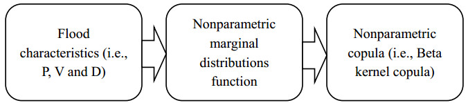
In this model simulation, best-fitted marginal distributions are modelled with nonparametric kernel density estimation procedure (see, Eq 6 of section 3.3.2) and their joint dependence structure are modelled using the nonparametric copula framework which is based on the Beta kernel function (see Eq 13) as referred by literatures such as Harrell and Davis ^[47], Brown and Chen ^[48], Chen ^[49] and Bounezmarni and Rombouts ^[50] (see Figure 3). The beta kernel estimators are free of boundary bias, non-negative and achieve the optimal rate of convergence for the mean integrated squared error. In other words, it can easily alleviate the severe boundary bias or can easily tackle the issue of boundary leakage problems which is often encountered in different standard kernel functions. Mathematically, if ${{\rm{U}}_1}, {\rm{}}{{\rm{U}}_2}, \ldots \ldots.., {{\rm{U}}_{\rm{n}}}{\rm{}}$ be the n^th set of uniform random observations with support in [0, 1], then the univariate Beta kernel function can be defined as;

Figure 3.  Operational flow diagram of Model type-1.

DownLoad: Full-Size Img PowerPoint

where, h is the bandwidth of kernel function; ${\rm{K}}\left({.{\rm{}}, {\rm{ \mathsf{ α} }}, {\rm{ \mathsf{ β} }}} \right)$ represents the Beta density function with parameters "${\rm{ \mathsf{ α} }}$" and "${\rm{ \mathsf{ β} }}$" and which can be mathematically formulated by;

According to Charpentier et al. ^[51], the Beta kernel copula can be incorporated to estimate bivariate copula density as defined by;

Therefore, for this model, using Eq 13 we can easily derive the joint PDFs and joint CDFs of the flood characteristics.

3.5.   Simulation of Model type-2 (parametric marginal distribution with nonparametric copula)

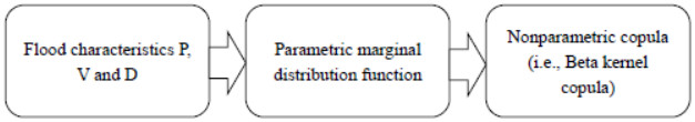
In this simulation approach (see Figure 4), the marginal distributions of flood characteristics are modelled with parametric families based probability functions (see, section 3.2.1) but their joint structure are still modelled under nonparametric copula framework using the Beta kernel copula (see Eq 13). As mentioned in the section 3.2.1, a distinguish varieties of parametric families functions are introduced and tested to define best-fitted marginal distribution of flood characteristics. Again, using the Eq 13 of the Beta kernel copula framework, we can easily modelled the joint behaviour of nonparametric marginal distributions and to derived the joint CDFs of the flood characteristics.

Figure 4.  Operational flow diagram of Model type-2.

DownLoad: Full-Size Img PowerPoint

4.   Results and discussions

4.1.   Modelling of parametric and nonparametric marginal distributions

Referred to section 3.2.1 and Table 2, a distinct variety of parametric functions are introduced as a candidate models and their parameters are estimated using the MLE, MOM, LS and L-moments algorithms and their estimated values are listed in Table 4. All the univariate distribution fitting procedures are carried out using the Easyfit-distribution fitting software. On the otherside, referred to section 3.2.2 and Table 3, five standard univariate kernel density functions are selected under nonparametric approximation and their bandwidth are estimated using the optimal bandwidth algorithm of Eq 7 and which is further employed for estimating the PDFs of individual flood characteristics. According to Kim et al. ^[52], the nonparametric density approximations didn't facilitate any closed form of the PDF and CDF thus, CDFs are estimated through the empirical procedure which is based on the numerical integration ^[25].

Table 4.  Estimated parameters of fitted probability distributions.

Kernel function	K(x)
Parametric Functions	Peak (P)	Volume (V)	Durations (D)
Gamma (2P)	a = 1.7166, b = 3540.6	a = 1.71, b = 11183.0	a = 3.0786, b = 6.1845
Gamma(3P)	a = 1.2106, b =4290, g = 884.47	a = 1.0848, b = 14723.0, g = 3150.8	a = 1.4696, b = 8.3319, g = 6.7958
GEV(3P)	k = 0.22596, s = 2683.6, m = 3765.6	k = 0.20446, s = 8736.0, m = 11890.0	k = 0.20682, s = 6.0766, m = 13.987
Log-Gamma(2P)	a = 129.15, b = 0.06544	a = 164.32, b = 0.05839	a = 35.165, b = 0.08037
Log-Logistic (2P)	a = 2.2801, b = 4541.7	a = 2.2731, b = 14202.0	a = 3.6928, b = 16.426
Log-Normal (2P)	s = 0.7362, m = 8.4513	s = 0.74093, m = 9.5943	s = 0.47178, m = 2.826
Weibull (2P)	a = 1.599, b = 6398.7	a = 1.5993, b = 20008.0	a = 2.5437, b = 20.375
Inverse. Gaussian (2P)	l = 10434.0, m = 6078.0	l = 32699.0, m = 19122.0	l = 58.617, m = 19.04
Johnson SB (4P)	g = 1.5161, d = 0.74495 l = 27319.0, x = 1304.2	g = 2.2027, d = 1.0357, l = 1.3052E+5, x = 961.8	g = 2.5314, d = 0.92215, l = 118.81, x = 8.2791

---

 | Show Table

DownLoad: CSV

The theoretical CDFs of each flood characteristics which are estimated through both parametric and nonparametric distribution framework are compared against empirical non-exceedance probabilities using the goodness-of fit test statistics (GOF), for outlining the data reproducing capabilities and fitness consistency level with the observational samples. The empirical observations are estimated using the Gringorten plotting position formulae (i.e., ^[7]) as given below;

where, "i" represents the smallest observations within the data sets of N observations when the data are arranged in ascending order. Several GOF test statistics are incorporated to measure the fitness level such as, error indices statistics called Mean square error (MSE) and Root mean square error (RMSE) (i.e., ^[22]), Kullback- Leibler information measures i.e., Kullback-Leibler (i.e., ^[53]) based information criteria statistics called the Akaike information criteria (AIC) (i.e., ^[54]), Schwartz's Bayesian information criteria (BIC) (i.e., ^[55]) and Hannan-Quinn Information criteria (HQC) (i.e., ^[56]), where the best-fitted univariate functions often signify for the minimum value of RMSE, MSE, AIC, BIC and HQC statistics, see Table 5a, b. Based on parametric modelling investigation, it reveals that the Lognormal-2P distribution are much satisfactory for flood peak samples, the Johnson SB (4P) for volume and Gamma(4P) distribution for duration series because these distribution possess minimum test statistics values such as for the flood peak series (AIC = −379.344, BIC = −375.52, HQC = −377.89, MSE = 0.00046 and RMSE = 0.02163 for the Lognormal (2P) distribution), for volume series (AIC = −381.821, BIC = −374.173, HQC = −378.9, MSE = 0.00041 and RMSE = 0.02028 for the Johnson SB (4P) distribution) and for duration series (AIC = −343.62, BIC = −337.88, HQC = −341.438, MSE = 0.000918 and RMSE = 0.030312 for the Gamma (3P) distribution) (referred to Table 5a, b). Similarly, for the nonparametric kernel density estimation procedure, the performance of Triweight kernel density function is much satisfactory for all the three flood characteristics i.e., flood peak, volume and duration series, as referred to Table 6 (indicated by bold letter). Overall, it is conclude that Lognormal (2P), Johnson SB (4P) and Gamma (3P) distribution are recognized as most justifiable for describing marginal distribution of flood peak, volume and duration series under parametric distribution framework on the otherside, the Triweight kernel function is recognized as most parsimonious for all the three flood characteristics.

Table 5a.  Performance measures based on (a) Information criteria statistics such as AIC, BIC & HQC.

Functions	Peak				Volume				Duration
	AIC	BIC	HQC		AIC	BIC	HQC		AIC	BIC	HQC
GEV(3P)	–374.335	–368.599	–372.15		–268.985	–263.249	–266.8		–336.32	–330.583	–334.135
Log-Gamma (2P)	–370.146	–366.322	–368.69		–359.914	–356.09	–358.46		–340.53	–336.709	–339.077
Log-Logistic (2P)	–360.392	–356.568	–358.94		–294.927	–291.103	–293.47		–321.32	–317.493	–319.861
Gamma (2P)	–335.861	–332.037	–334.4		–360.025	–356.201	–358.57		–260.55	–256.722	–259.089
Gamma (3P)	–216.301	–210.565	–214.12		–210.107	–204.371	–207.92		–343.62	–337.88	–341.438
Log-Normal (2P)	–379.344	–375.52	–377.89		–371.028	–367.204	–369.57		–327.46	–323.633	–326.001
Weibull (2P)	–329.681	–325.857	–328.23		–342.868	–339.044	–341.41		–292.91	–289.085	–291.453
Inv. Gaussian (2P)	–362.489	–358.665	–361.03		–344.722	–340.898	–343.27		–325.76	–321.938	–324.306
Johnson SB(4P)	–340.899	–333.251	–337.99		–381.821	–374.173	–378.91		–223.65	–216.006	–220.742
Notes: AIC stands for Akaike information criteria; BIC stands for Bayesian information criteria; HQIC or HQC stands for Hannan-Quinn information criteria.

---

 | Show Table

DownLoad: CSV

Table 5b.  Performance measures based on error indices statistics such as MSE and RMSE.

	Peak			Volume			Duration
Functions	MSE	RMSE		MSE	RMSE		MSE	RMSE
GEV(3P)	0.00049	0.02229		0.00409	0.06394		0.00106	0.03261
Log-Gamma(2P)	0.00056	0.02372		0.00069	0.02627		0.0010172	0.031894
Log-Logistic(2P)	0.00068	0.02615		0.00253	0.05032		0.00149	0.03865
Gamma(2P)	0.00111	0.03341		0.00068	0.02624		0.005037	0.070973
Gamma(3P)	0.01173	0.10882		0.01327	0.11520		0.000918	0.030312
Log-Normal(2P)	0.00046	0.02163		0.00055	0.02351		0.001321	0.03635
Weibull(2P)	0.00126	0.03555		0.00097	0.03115		0.002637	0.05135
Inv. Gaussian(2P)	0.00066	0.02561		0.00094	0.03059		0.00137	0.03697
Johnson SB (4P)	0.00093	0.03053		0.00041	0.02028		0.00972	0.09861
Notes. MSE stands for Mean square error; RMSE stands for Root mean square error.

---

 | Show Table

DownLoad: CSV

Table 6.  Performance measures of the fitted nonparametric kernel functions.

Flood characteristics	F(X)	Error indices statistics			Information criteria statistics
		MSE (or Mean square error)	RMSE (or Root mean square error)		AIC (or Akaike information criteria)	BIC (or Bayesian information criteria)	HQC (or Hannan-Quinn Information criteria)
P	Epanechnikov	0.00038	0.01957		−391.37	−389.45	−390.64
	Bi-weight or quartic	0.00026	0.01620		−410.25	−408.34	−409.52
	Triweight	0.00022	0.01483		−419.07	−417.16	−418.34
	Triangular	0.00028	0.01686		−406.26	−404.35	−405.54
	Cosine	0.00032	0.01800		−399.98	−398.07	−399.25
V	Epanechnikov	0.00093	0.03060		−346.66	−344.75	−345.93
	Bi-weight or quartic	0.00018	0.01350		−428.44	−426.53	−427.71
	Triweight	0.00016	0.01287		−433.27	−431.36	−432.55
	Triangular	0.00020	0.01426		−423.01	−421.10	−422.29
	Cosine	0.00022	0.01514		−417.02	−415.11	−416.30
D	Epanechnikov	0.00059	0.02430		−369.69	−367.77	−368.96
	Bi-weight or quartic	0.00051	0.02265		−376.71	−374.80	−375.99
	Triweight	0.00048	0.02208		−379.27	−377.36	−378.54
	Triangular	0.00055	0.02357		−372.74	−370.83	−372.01
	Cosine	0.00062	0.02496		−367.03	−365.12	−366.30

---

 | Show Table

DownLoad: CSV

4.2.   Analysis of Model type-1 and Model type-2

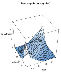
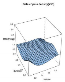
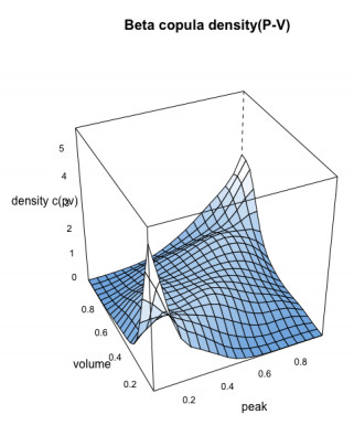
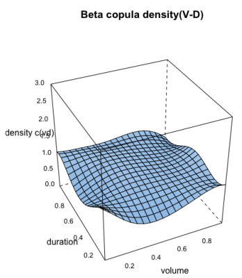
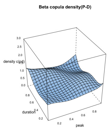
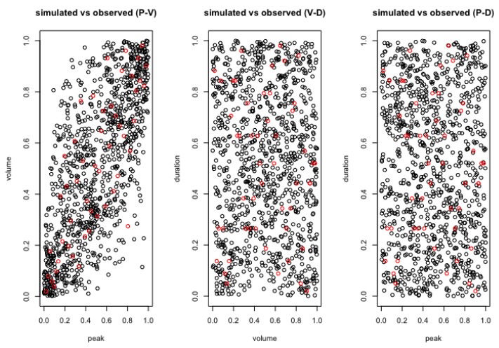
In the simulation of Model type-1, the best-fitted marginal distributions which are selected under the nonparametric distribution framework (see, section 4.1) i.e., the Triweight kernel density function for the each individual flood characteristics are introduced into the nonparametric copula framework called the Beta kernel copula density (see section 3.4) and using Eq 13 with the uniform variables generated using the Triweight kernel functions, we estimated the bivariate copula density and joint cumulative distribution function (or JCDFs) for flood peak-volume, volume-duration and peak-duration pairs. Figures 5–7 illustrated the bivariate beta copula density function of flood peak-volume, volume-duration and peak-duration pairs also, Figure 8, represents the comparison between simulated (indicated by black colour) flood samples deriving from the beta kernel copula density and the observed (indicated by red colour) flood characteristics.

Figure 5.  Bivariate beta copula density of flood peak-volume series using Model type-1.

DownLoad: Full-Size Img PowerPoint

Figure 6.  Bivariate beta copula density of flood volume-duration pair using Model type-1.

DownLoad: Full-Size Img PowerPoint

Figure 7.  Bivariate beta copula density of flood peak-duration pair using Model type-1.

DownLoad: Full-Size Img PowerPoint

Figure 8.  Comparison between the simulated (black colour) flood samples derived from beta copula density using Model type-1 and observed (red colour) flood samples.

DownLoad: Full-Size Img PowerPoint

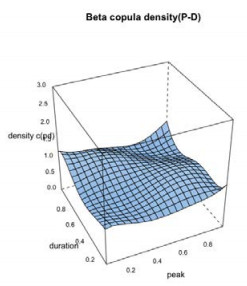
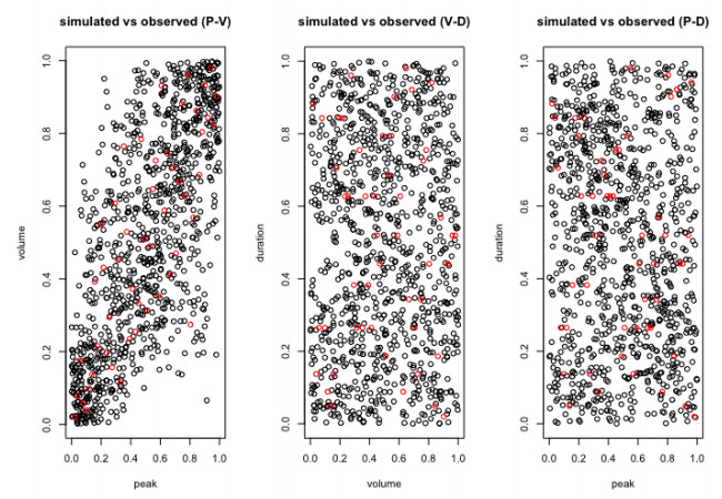
Similarly, for the Model type-2, the bivariate beta kernel copula densities for flood characteristics are estimated using the same Eq 13 with the uniform flood variables which are generated using the Lognormal (2P) and Johnson SB (4P) for flood peak-volume pair, the Johnson SB (4P) and Gamma (3P) for flood volume-duration pair and the Lognormal (2P) and Gamma (3P) distributions for flood peak-duration pair. Figures 9–11, illustrated the bivariate beta copula density function with parametric marginal distribution of the flood peak-volume, volume-duration and peak-duration pairs also, Figure 12 represented the comparison between simulated (indicated by black colour) flood samples derived from the beta kernel copula density and the observed (indicated by red colour) flood characteristics.

Figure 9.  Bivariate beta copula density of flood peak-volume pair using Model type-2.

DownLoad: Full-Size Img PowerPoint

Figure 10.  Bivariate beta copula density of flood volume and duration series using Model type-2.

DownLoad: Full-Size Img PowerPoint

Figure 11.  Bivariate beta copula density of flood peak-duration pair using Model type-2.

DownLoad: Full-Size Img PowerPoint

Figure 12.  Comparison between simulated (black colour) samples derived from beta copula density function using Model 2 and observed (red colour) flood samples.

DownLoad: Full-Size Img PowerPoint

4.3.   Estimation of return periods

4.3.1.   Univariate return periods

In hydrological planning and design, the hydrologist or water practioner are often interested in the evaluation of the mean inter-arrival period between two design events which usually defined in a year called the return period ^[18,57]. The basic concept of return periods are thoroughly discussed by Yue and Rasmussen (i.e., ^[37]) and Salvadori and De Michele (i.e., ^[19]). Mathematically, the univariate return period of the targeted flood characteristics that occurs once in a year are estimated from the univariate cumulative distribution function or CDF of flood characteristics (say "X") as given below:

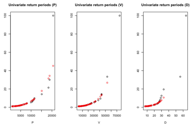
where μ is the mean inter-arrival time between two consecutive flood episodes and that could be equal to unity (i.e., μ = 1) for annual maxima based flood modelling (i.e., ^[37]). Figure 13 represented the univariate return periods derived from the best-fitted parametric and nonparametric marginal distribution functions of the flood characteristics.

Figure 13.  Univariate return periods derived from the best-fitted parametric (red colour) and nonparametric (black colour) marginal distribution of flood characteristics.

DownLoad: Full-Size Img PowerPoint

4.3.2.   Bivariate joint return periods

An effective risk analysis often demands the accountability of multiple potential flood characteristics based on joint probability density function or JPDF and joint cumulative distribution functions or JCDF ^[18,19,58]. Actually, the selection of return periods is depending upon the importance of undertaken structure as well as its consequences of failure where, their appropriate selection often attributed an impact over the strength of design variables quantiles ^[58]. The joint probability distribution can be describe through two different approach such that in the first condition both the flood variables (say, ${\rm{P}} \ge {\rm{p}}$ AND ${\rm{V}} \ge {\rm{v}}$) simultaneously exceed certain threshold during a flood events and their associated return period called AND joint period and it can be written in the form of;

where ${\rm{H}}\left({{\rm{p}}, {\rm{v}}} \right)$ is the JCDF between flood variable (say, P and V) that can be expressed in the context of bivariate Copula function C(F(p), F(v)); F(p) and F(v) best-fitted marginal distribution of the flood characteristics P and V. Similarly, in the second situation, the probability either the first or second flood variable (say, ${\rm{P}} \ge {\rm{p}}$ OR ${\rm{V}} \ge {\rm{v}}$) exceed given threshold and thus their associated return period called OR joint return period and can be expressed as;

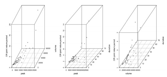
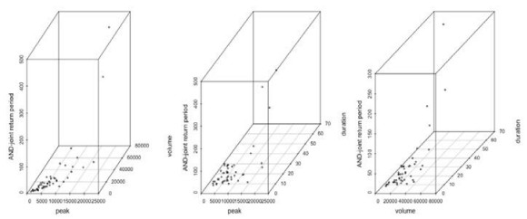
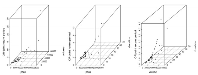
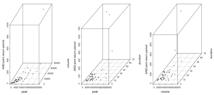
Therefore, using Eqs 16 and 17, the joint return periods between flood peak-volume, volume-duration and peak-duration pairs for the "AND" and "OR" joint cases are estimated and their values for few flood combinations are listed in the Tables 7 and 8. Figures 14 and 15 illustrated the estimated "OR" and "AND" joint return periods between peak-volume, volume-duration and peak-duration for the Model type-1. Similarly, the graphical illustration of the "OR" and "AND" joint return periods for Model type-2 are presented in Figures 16 and 17. Based on the estimated joint return periods (referred to Tables 7 and 8), it is concluded that the OR-joint return period is smaller than AND-joint return periods for different possible combination of the flood characteristics i.e., ${\rm{T}}_{{\rm{PV}}}^{{\rm{OR}}} < {\rm{T}}_{{\rm{AND}}}^{{\rm{OR}}}$. For example, a flood episode, i.e., P = 10463.8 m³s⁻¹, V = 17148 m³ and D = 29 days, the OR-joint return period between P-V, T_PV^OR = 2.183323266 years, between P-D, T_PD^OR = 4.11086032 years, and between V-D is, T_VD^OR = 2.03275 years, derived from Model type-1. Similarly, for the same flood combination and same Model type-1, the AND-joint return period is T_PV^AND = 7.02902155 years, T_PD^AND = 50.702086 years and T_VD^AND = 24.4200621 years. Similarly, for the flood episodes P = 20586.4, m³s⁻¹, V = 43273.2 m³ and D = 7 days, the OR-joint return period between P-V, T_PV^OR = 11.100995 years, between P-D, T_PD^OR = 1.00312117 years, and between V-D is, T_VD^OR = 1.00290911 years based on the Model type-2. Also, for both the Model type-1 and Model type-2, for example from Table 7, the univariate return periods derived from flood peak flow, T(P) or volume series, T(V) produces high return periods than derived from their joint associations for "OR" cases i.e., T(P) > T(V) > T_PV^OR. Similarly, the return periods derived from flood volume, T(V) and duration series, T(D) produces high return periods than derived from "OR" joint cases between volume-duration pairs, i.e., T(V) > T(D) > T_VD^OR. Also, the return periods derived from flood peak, T(P) and duration series, T(D) generated higher return periods than return periods for OR-joint cases, i.e., T(P) > T(D) > T_PD^OR. Similarly, the same mathematical inequalities are exhibited between univariate and bivariate return periods derived from the Model type-2.

Table 7.  Univariate and Bivariate joint return derived from the Model type-1.

P	V	D	T(P)	T(V)	T(D)	TPVOR	TPDOR	TVDOR	TPVAND	TPDAND	TVDAND
10436.8	17148	29	6.053	2.298	10.225	2.183	4.110	2.03	7.029	50.702	24.420
20586.4	43273.2	7	100	13.765	1.0279	12.548	1.027	1.025	338.580	104.788	14.260
11192.4	21994.2	30	8.118	3.347	12.610	3.079	5.270	2.805	10.294	78.495	46.272
9929.3	9667.4	56	5.402	1.402	33.333	1.387	4.815	1.386	5.643	134.531	46.571
7686.9	41309	19	4.031	9.445	2.456	3.533	1.763	2.094	14.111	11.360	28.132
5052.6	19073.8	64	2.131	2.769	100	1.822	2.109	2.720	3.552	190.669	281.210
18339.4	74740	16	21.428	100	1.980	18.361	1.886	1.959	453.389	46.333	224.181

---

 | Show Table

DownLoad: CSV

Table 8.  Univariate and Bivariate joint return periods derived from the Model type-2.

P	V	D	T(P)	T(V)	T(D)	TPVOR	TPDOR	TVDOR	TPVAND	TPDAND	TVDAND
10436.8	17148	29	7.243	2.329	6.969	2.224	3.861	1.944	8.487	44.294	17.102
20586.4	43273.2	7	45.206	13.394	1.003	11.100	1.003	1.002	149.285	45.491	13.457
11192.4	21994.2	30	8.460	3.219	7.736	2.981	4.359	2.478	10.712	55.281	27.481
9929.3	9667.4	56	6.513	1.424	131.578	1.408	6.268	1.420	6.871	625.302	187.388
7686.9	41309	19	3.995	11.715	2.550	3.604	1.802	2.221	17.180	11.439	36.619
5052.6	19073.8	64	2.180	2.649	322.580	1.812	2.172	2.635	3.514	627.012	911.610
18339.4	74740	16	31.434	149.925	1.928	26.730	1.870	1.914	932.964	62.583	324.412

---

 | Show Table

DownLoad: CSV

Figure 14.  OR-joint return periods derived from Model type-1(i.e., nonparametric marginal distribution modelled with nonparametric copula function called Beta kernel copula).

DownLoad: Full-Size Img PowerPoint

Figure 15.  AND-joint return periods derived from the Model type-1.

DownLoad: Full-Size Img PowerPoint

Figure 16.  OR-joint return periods derived from the Model type-2 (i.e., parametric marginal distribution modelled with nonparametric copula function called Beta kernel copula).

DownLoad: Full-Size Img PowerPoint

Figure 17.  AND-joint return periods derived from the Model type-2.

DownLoad: Full-Size Img PowerPoint

4.3.3.   Conditional return periods

In most of the hydrological design requirements, it is often an essential concern to demonstrate flood events through highlighting the priority of one over the another design variables. Thus, several literature pointed out the necessity of conditional distribution for defining the concept of conditional return periods such as Salvadori and De Michele ^[19], Shiau ^[46], Zhang and Singh ^[7], Brunner et al., ^[58]. The conditional return relies on the conditional relationship between flood characteristics given that some condition is fulfilled. Mathematically, the conditional return periods of flood peak given various percentile value of flood volume or vice-versa or in another words, where the flood peak "P" exceeds a threshold "p" given that the volume "V" exceeds a threshold "v" can be expressed as;

Overall, using the above Eq 19, the return periods of one variable conditioning to another variable for any possible combination of flood characteristics are estimated and their values for few combinations are listed in Tables 9 and 10, derived from the Model type-1 and Model type-2. For example, a flood episode with peak flow, P = 10463.8 m³s⁻¹, volume, V = 17148 m³ and duration, D = 29 (days), the joint return period of, "P" conditional to "V" is ${\rm{T}}\left({{\rm{p}}\backslash {\rm{V}} \le {\rm{v}}} \right){\rm{}}$ = 24.647 years; "P" conditioning to "D" is ${\rm{T}}\left({{\rm{p}}\backslash {\rm{D}} \le {\rm{d}}} \right)$ = 6.202 years; and "V" conditioning to "D" is ${\rm{T}}\left({{\rm{v}}\backslash {\rm{D}} \le {\rm{d}}} \right)$ = 2.289 years. On the other side, for the Model type-2, a flood episode characterized with peak flow, P = 10463.8 m³s⁻¹, volume, V = 17148 m³ and duration, D = 29 (days), then the return period of 'P' conditioning to "V" is ${\rm{T}}\left({{\rm{p}}\backslash {\rm{V}} \le {\rm{v}}} \right){\rm{}}$ = 28.195 years, "P" conditioning to "D" is ${\rm{T}}\left({{\rm{p}}\backslash {\rm{D}} \le {\rm{d}}} \right)$ = 7.417 years and "V" conditioning to "D" is ${\rm{T}}\left({{\rm{v}}\backslash {\rm{D}} \le {\rm{d}}} \right) =$ 2.309 years.

Table 9.  Conditional joint return periods derived from the Model type-1.

P	V	D	${\rm{T}}\left({{\rm{P}}/{\rm{V}} \le {\rm{v}}} \right)$	${\rm{T}}\left({{\rm{V}}/{\rm{P}} \le {\rm{p}}} \right)$	${\rm{T}}\left({{\rm{P}}/{\rm{D}} \le {\rm{d}}} \right)$	${\rm{T}}\left({{\rm{D}}/{\rm{P}} \le {\rm{p}}} \right)$	${\rm{T}}\left({{\rm{V}}/{\rm{D}} \le {\rm{d}}} \right)$	${\rm{T}}\left({{\rm{D}}/{\rm{V}} \le {\rm{v}}} \right)$
10436.8	17148	29	24.647	2.850	6.202	10.692	2.289	9.937
20586.4	43273.2	7	131.605	14.205	59.429	1.027	10.776	1.027
11192.4	21994.2	30	26.938	4.349	8.337	13.173	3.322	12.156
9929.3	9667.4	56	36.244	1.521	5.459	36.110	1.402	33.669
7686.9	41309	19	5.047	21.478	3.705	2.356	8.429	2.406
5052.6	19073.8	64	3.403	6.669	2.133	111.611	2.768	99.146
18339.4	74740	16	22.266	122.310	19.738	1.972	89.385	1.978

---

 | Show Table

DownLoad: CSV

Table 10.  Conditional joint return periods derived from the Model type-2.

P	V	D	${\rm{T}}\left({{\rm{P}}/{\rm{V}} \le {\rm{v}}} \right)$	${\rm{T}}\left({{\rm{V}}/{\rm{P}} \le {\rm{p}}} \right)$	${\rm{T}}\left({{\rm{P}}/{\rm{D}} \le {\rm{d}}} \right)$	${\rm{T}}\left({{\rm{D}}/{\rm{P}} \le {\rm{p}}} \right)$	${\rm{T}}\left({{\rm{V}}/{\rm{D}} \le {\rm{d}}} \right)$	${\rm{T}}\left({{\rm{D}}/{\rm{V}} \le {\rm{v}}} \right)$
10436.8	17148	29	28.195	2.766	7.417	7.128	2.309	6.712
20586.4	43273.2	7	60.001	14.388	23.458	1.003	9.303	1.003
11192.4	21994.2	30	27.747	4.059	8.697	7.931	3.175	7.423
9929.3	9667.4	56	37.203	1.521	6.531	141.059	1.424	131.699
7686.9	41309	19	4.762	27.611	3.733	2.461	10.472	2.507
5052.6	19073.8	64	3.574	5.824	2.180	359.637	2.648	310.782
18339.4	74740	16	32.313	172.947	30.400	1.926	134.173	1.926

---

 | Show Table

DownLoad: CSV

5.   Conclusions

The joint distribution analysis between the multiple interacting flood characteristics is an essential concern for a better understanding of critical hydrologic behaviour of flood episodes. In this demonstration, a nonparametric copula-based multivariate flood distribution modelling are conducted and applied as a case study for the Kelantan River basin at Gulliemard bridge gauge station in Malaysia. In this experiment two different modelling framework are constructed such that in the Model-type-1, the best-fitted marginal distribution of each individual flood characteristics are modelled with nonparametric kernel density estimation procedure and their joint dependence structure are modelled using nonparametric copula which is based on the Beta kernel function where, the Beta kernel copula function is incorporated to estimate the bivariate copula density between flood peak-volume, volume-duration and peak-duration pairs. On the other side, in the construction of second Model type-2, the marginal distributions of the flood characteristics are modelled with parametric families based probability distribution functions and their joint structure are still modelled under nonparametric copula framework using the same Beta kernel copula.

In the simulation of Model type-1, a set of five standard univariate kernel functions are introduced and their bandwidth are estimated using the optimal bandwidth algorithm. Based on several goodness-of-fit test statistics, referred to Table 6, the Triweight kernel function is recognized as most justifiable for describing marginal distribution of flood peak, volume and duration series under nonparametric distribution framework. Finally, the Beta kernel copula density are estimated using the Eq 13 with the uniform variables which are derived from the best-fitted flood marginal distribution (i.e., Triweight kernel density function) and to derived the joint CDFs of flood peak-volume, volume-duration and peak-duration series. Similarly, for the Model type-2, an interactive sets of parametric families-based probability functions are introduced as a candidate models and their parameters are estimated using the maximum likelihood estimation (MLE), method of moments, least square method (LS), and L statistics-based method of L-moments. Based on several goodness-of-fit test statistics i.e., MSE, RMSE, AIC, BIC and HQC statistics, the Lognormal (2P), Johnson SB (4P) and Gamma (3P) distribution are recognized as most justifiable for describing marginal distribution of flood peak, volume and duration series under parametric distribution framework. Finally, the Beta kernel copula density are estimated using the Eq 13 with the uniform variables which are derived from the best-fitted flood marginal distribution and to derived the joint CDFs of flood characteristics. The JCDF of flood peak-volume, volume-duration and peak-duration pairs are employed to derived the joint and conditional return periods. Overall, based on the above simulations it could be concluded that the nonparametric distribution framework which are implemented in this literature could be applicable for analysing hydrologic behaviour i.e., flood modelling or rainfall modelling in most part of the world.

Acknowledgements

Special thanks is extended to the Drainage and Irrigation Department, Malaysia for supplying streamflow data of the Kelantan river basin.

Funding Acknowledgements: The author(s) received no financial support for the research, authorship, and/or publication of this article.

Conflict of interest

All authors declare no conflicts of interest in this manuscript.