Existence, uniqueness and numerical solution of stochastic fractional differential equations with integer and non-integer orders

Seda IGRET ARAZ; Mehmet Akif CETIN; Abdon ATANGANA; Seda IGRET ARAZ; Mehmet Akif CETIN; Abdon ATANGANA

doi:10.3934/era.2024035

Electronic Research Archive

2024, Volume 32, Issue 2: 733-761. doi: 10.3934/era.2024035

Previous Article Next Article

Research article Special Issues

Existence, uniqueness and numerical solution of stochastic fractional differential equations with integer and non-integer orders

1.
Siirt University, Department of Mathematics Education, Siirt, Turkey
2.
Institute for Groundwater Studies, Faculty of Natural and Agricultural Sciences, University of the Free State, South Africa
3.
ALTSO Vocational School, Alanya Alaaddin Keykubat University, Antalya, Turkey
4.
Department of Medical Research, China Medical University Hospital, China Medical University, Taichung, Taiwan
5.
IT4Innovations, VSB–Technical University of Ostrava, Ostrava-Poruba 70800, Czech Republic

Received: 26 September 2023 Revised: 03 December 2023 Accepted: 15 December 2023 Published: 10 January 2024

The parametrized approach is extended in this study to find solutions to differential equations with fractal, fractional, fractal-fractional, and piecewise derivatives with the inclusion of a stochastic component. The existence and uniqueness of the solution to the stochastic Atangana-Baleanu fractional differential equation are established using Caratheodory's existence theorem. For the solution of differential equations using piecewise differential operators, which take into account combining deterministic and stochastic processes utilizing certain significant mathematical tools such as fractal and fractal-fractional derivatives, the applicability of the parametrized technique is being examined. We discuss the crossover behaviors of the model obtained by including these operators and we present some illustrative examples for some problems with piecewise differential operators.

Keywords:

Citation: Seda IGRET ARAZ, Mehmet Akif CETIN, Abdon ATANGANA. Existence, uniqueness and numerical solution of stochastic fractional differential equations with integer and non-integer orders[J]. Electronic Research Archive, 2024, 32(2): 733-761. doi: 10.3934/era.2024035

Related Papers:

[1]	Colin Klaus, Matthew Wascher, Wasiur R. KhudaBukhsh, Grzegorz A. Rempała . Likelihood-Free Dynamical Survival Analysis applied to the COVID-19 epidemic in Ohio. Mathematical Biosciences and Engineering, 2023, 20(2): 4103-4127. doi: 10.3934/mbe.2023192
[2]	Marcin Choiński, Mariusz Bodzioch, Urszula Foryś . A non-standard discretized SIS model of epidemics. Mathematical Biosciences and Engineering, 2022, 19(1): 115-133. doi: 10.3934/mbe.2022006
[3]	Maghnia Hamou Maamar, Matthias Ehrhardt, Louiza Tabharit . A nonstandard finite difference scheme for a time-fractional model of Zika virus transmission. Mathematical Biosciences and Engineering, 2024, 21(1): 924-962. doi: 10.3934/mbe.2024039
[4]	Yong Yang, Zunxian Li, Chengyi Xia . Forced waves and their asymptotic behaviors in a Lotka-Volterra competition model with spatio-temporal nonlocal effect under climate change. Mathematical Biosciences and Engineering, 2023, 20(8): 13638-13659. doi: 10.3934/mbe.2023608
[5]	Sai Zhang, Li Tang, Yan-Jun Liu . Formation deployment control of multi-agent systems modeled with PDE. Mathematical Biosciences and Engineering, 2022, 19(12): 13541-13559. doi: 10.3934/mbe.2022632
[6]	A Othman Almatroud, Noureddine Djenina, Adel Ouannas, Giuseppe Grassi, M Mossa Al-sawalha . A novel discrete-time COVID-19 epidemic model including the compartment of vaccinated individuals. Mathematical Biosciences and Engineering, 2022, 19(12): 12387-12404. doi: 10.3934/mbe.2022578
[7]	Jianquan Li, Zhien Ma, Fred Brauer . Global analysis of discrete-time SI and SIS epidemic models. Mathematical Biosciences and Engineering, 2007, 4(4): 699-710. doi: 10.3934/mbe.2007.4.699
[8]	Ziqiang Cheng, Jin Wang . Modeling epidemic flow with fluid dynamics. Mathematical Biosciences and Engineering, 2022, 19(8): 8334-8360. doi: 10.3934/mbe.2022388
[9]	Dimitri Breda, Davide Liessi . A practical approach to computing Lyapunov exponents of renewal and delay equations. Mathematical Biosciences and Engineering, 2024, 21(1): 1249-1269. doi: 10.3934/mbe.2024053
[10]	Sarah Treibert, Helmut Brunner, Matthias Ehrhardt . A nonstandard finite difference scheme for the SVICDR model to predict COVID-19 dynamics. Mathematical Biosciences and Engineering, 2022, 19(2): 1213-1238. doi: 10.3934/mbe.2022056

Abstract

1. Introduction

In recent times, academics have been increasingly interested in finding analytical solutions to some nonlinear partial differential equations that describe and model various physical and engineering problems, including fluid dynamics, plasma astrophysics, ocean engineering, and nonlinear optics ^{[1,2,3,4,5,6]}. These equations function as mathematical representations that encapsulate the complexities of intricate physical occurrences. These models have broad applications in various nonlinear scientific fields such as fluid mechanics, biology, chemistry, physics, plasmas, and optical fibers. Their applicability highlights their relevance in explaining and forecasting the behavior of complex systems across various scientific fields. To better understand the dynamics of these real-world components, methods for solving fractional nonlinear partial differential equations (PDEs) must be investigated ^{[7,8,9,10,11]}. This exploration is necessary to study and understand the complex behaviors inherent in the systems above. Solutions to nonlinear fractional PDEs (FPDEs) are of academic interest because of the increased detail and generality they provide, as they outperform traditional solutions in terms of descriptive power. In addition to improving our understanding and predictive capabilities in these vital areas of nonlinear physics, this study has implications for a wide range of real-world applications because it clarifies nonlinear aspects. Researchers in the field of nonlinear physics have significantly contributed to our knowledge of complex processes in various other scientific fields ^{[12,13,14,15,16]}.

The investigation of analytical solutions for FPDEs is intrinsically tricky, and it has led to the creation of many mathematical strategies to address this complex issue. Because analytical solutions can offer a comprehensive understanding of fundamental physical processes and show the precise behavior of the modeled system beyond what can be achieved by using numerical approaches, analysts are particularly drawn to them. Consequently, pursuing analytical solutions for FPDEs is recognized as a crucial and continuously developing field of study ^[17,18,19]. Various mathematical techniques have been employed in scholarly literature to solve different types of FPDEs efficiently and analytically ^{[20,21,22,23,24]}. This demonstrates the extensive scope of research in this field. Numerous strategies have been employed, showing the diversity of approaches that researchers in this discipline have chosen ^[25,26,27]. Among the approaches under consideration, several techniques ^{[28,29,30,31,32,33,34,35,36]} have emerged as noteworthy contributors. Every approach has unique benefits, broadening the toolkit of techniques that can be used to solve FPDEs and improving our understanding of these complex mathematical models ^[37,38].

Furthermore, integrated into the structure of the suggested methodology, the Riccati-Bernoulli sub-optimal differential equation (ODE) method ^[39,40,41] is a powerful tool. It is well known for its adept management of complex algebraic calculations and ability to derive solutions for a wide range of phenomena that occur in applications such as biology, chemistry, physics, fluid mechanics, and optical fibers. This methodology has significant potential for use in several scientific and engineering fields. Its application in the fields of biological systems, industrial operations, and environmental flows can facilitate a deep understanding of the complexities of fluid behavior, thereby improving optimization and forecasting methods. The FPDEs are transformed into an algebraic system by using the Bäcklund transformation and the Riccati-Bernoulli equation, simplifying the extraction of important information from the intricate dynamics present in these systems. This method greatly enhances our understanding of the underlying physical mechanisms. The methodology is particularly noteworthy because it guarantees the derivation of finite solutions, thereby validating the precision and effectiveness of solutions for the equations under examination. A critical feature of this approach is its potential to produce a wide range of single-wave solutions, increasing its adaptability and usefulness.

Moreover, the current study was designed to utilize an analytical approach to clarify the complex dynamics of the Dullin-Gottwald-Holm (DGH) equation ^[42]. This study also looks at how linear dispersion parameters change the shape of traveling waves that are connected to the DGH equation and the isospectral features of soliton solutions. It should be mentioned here that the DGH equation was derived from asymptotic expansions applied directly to the Hamiltonian driving Euler equations, and it was first developed as a model for unidirectional shallow water waves over a flat bottom

$\begin{equation} F_{t}+\lambda F_{x}+3FF_{x}-\mu^{2}\left( F_{xxt}+FF_{xxx}+2F_{x} F_{xx}\right) +\chi F_{xxx} = 0. \end{equation}$

(1.1)

The DGH equation is linked to two distinct soliton equations that govern water waves and can be integrated independently. The DGH equation (1.1) specifically can be reduced to the well-known Korteweg-de Vries (KdV) equation for ( $\mu = 0$ ) and ( $\chi\neq0$ ): $F_{t}+\lambda F_{x}+3FF_{x}+\chi F_{xxx} = 0$ . In contrast, the DGH equation (1.1) can be reduced to the Camassa-Holm (CH) equation for ( $\mu = 1$ ) and ( $\chi = 0$ ): $F_{t}+\lambda F_{x}+3FF_{x}-\left(F_{xxt}+FF_{xxx}+2F_{x}F_{xx}\right) = 0$ . This two-way connection shows how the DGH equation can be used to describe different wave events and how it can be used to combine the dynamics given by the KdV and CH equations in certain parameter situations. Numerous studies have been carried out to clarify the DGH equation of integer order. Dullin et al. ^[43] revealed another integrable instance in the DGH formula. A thorough treatment of the Cauchy problem related to the DGH equation was conducted in a different study ^[44]. Tang and Yang ^[45] extended the peakon equations by introducing an integral constant and using the dynamical systems bifurcation approach. Chen et al. ^[46] used the Darboux transformation technique to produce numerous soliton solutions. Zhang et al. ^[47] focused on peakons and periodic cusp wave solutions for a generalized CH equation by using the bifurcation theory of planar dynamical systems. Liu ^[48] explored questions about the creation of singularities and the existence of global solutions. Under the condition that $\mu^{2} < 0$ , Dullin et al. ^[49] showed that there are three different kinds of limited waves for the DGH equation. These different studies contribute to the development of a more thorough knowledge of the complex dynamics of the DGH equation for various parameter values. Regarding tasks that involve obtaining a precise description of complex nonlinear systems in a variety of scientific fields, such as fluid dynamics and oceanography, nonlinear dynamics and soliton theory, mathematical physics, numerical simulations, computational mathematics, and engineering, the fractional DGH equation is considered to be an essential tool to describe systems that display complex structures and subtle nonlinearities. The fractional DGH equation has the following mathematical expression:

$\begin{align} & (D_{t}^{\alpha}(F))+\lambda D_{x}^{\beta}(F)+3FD_{x}^{\beta}(F)\\ & \left. -\mu^{2}\left( D_{t}^{\alpha}(D_{x}^{2\beta}(F))+FD_{x}^{3\beta }(F)+2D_{x}^{\beta}(F)D_{x}^{2\beta}(F)\right) +\chi D_{x}^{3\beta }(F) = 0,\right. \end{align}$

(1.2)

with $0 < \alpha, \beta, \leq1$ , where $\alpha$ and $\beta$ indicate the time- and space-fractional parameters, respectively.

The height of the free surface over a flat bottom is represented by the function $F(x, t)$ , and the coefficient ( $\chi)$ indicates the linear dispersive parameter and the linear wave speed for undisturbed water at rest at spatial infinity is represented by ( $\lambda = 2\omega = \sqrt{gh}$ ). Here, ( $g$ ) indicates the gravitational constant, ( $h$ ) denotes the mean fluid depth, and ( $\omega$ ) represents the essential shallow water speed for undisturbed water at rest at spatial infinity. The Greek symbol ( $\mu^{2}$ ) represents square length scales. The operator representing the order $\alpha$ derivatives adheres to the definition provided in ^[50]:

$\begin{equation} D_{\theta}^{\alpha}{q(\theta)} = \lim\limits_{m\rightarrow0}\frac{q(m(\theta )^{1-\alpha}-q{(\theta)})}{m},0 < \alpha\leq1. \end{equation}$

(1.3)

This inquiry utilizes the following characteristics of this derivative:

$\begin{equation} \left\{ \begin{array} [c]{c} D_{\theta}^{\alpha}\left( j_{1}\eta(\theta)\pm j_{2}m(\theta)\right) = j_{1}D_{\theta}^{\alpha}(\eta(\theta))\pm j_{2}D_{\theta}^{\alpha} (m(\theta)),\\ D_{\theta}^{\alpha}\chi\left[ \xi^{\tau}(\theta)\right] = \chi_{\xi}^{\prime }(\xi(\theta))D_{\theta}^{\alpha}\xi(\theta). \end{array} \right. \end{equation}$

(1.4)

Hence, the primary motivation and goal of this investigation is to use the Riccati-Bernoulli sub-ODE method with the help of the Bäcklund transformation in order to analyze and solve the fractional DGH equation, as this method has not been used before to analyze this equation. We study how linear dispersion factors affect the shape of traveling waves in the DGH equation and look into the isospectral properties of soliton solutions. Through these analyses, our research advances knowledge by revealing new perspectives on the fundamental mechanisms underlying complicated occurrences, thus positioning itself as a ground-breaking undertaking in the scientific debate.

A meticulous and systematic approach has been adopted to structure the manuscript. A detailed exposition of the methods employed in Section 2 serves to elucidate the intricacy of the approach. Section 3 meticulously outlines the process of problem execution by using the described methodology. Section 4 offers a comprehensive discussion and synthesis of the results. Finally, Section 5 provides a succinct summary of the study's definitive findings and their broad implications.

2. Methodology

The FPDE described herein warrants consideration:

$\begin{equation} P_{1}\left( f,D_{t}^{\alpha}(f),D_{\zeta_{1}}^{\beta}(f),D_{\zeta_{2} }^{2\beta}(f),fD_{\zeta_{1}}^{\beta}(f),\ldots\right) = 0,\quad0 < \alpha ,\beta,\leq1. \end{equation}$

(2.1)

The polynomial $P_{1}$ is a function of $f(\zeta_{1}, \zeta_{2}, \zeta _{3}, ......, t)$ . This polynomial includes the fractional order derivatives as well as the nonlinear terms. The fundamental phases of this approach are then comprehensively addressed. The subsequent wave transformations are our recommendations for investigating potential solutions for Eq (1.2):

$\begin{equation} {F(x,t) = e^{i\psi}f(\psi),} \end{equation}$

(2.2)

with

$\begin{equation} \psi(x,t) = \left( {\frac{{x}^{\beta}}{\beta}}\right) -\kappa\left( {\frac{{t}^{\alpha}}{\alpha}}\right) . \end{equation}$

(2.3)

The function $\psi\equiv\psi\left(x, t\right)$ represents the transformation of propagating waves. The non-zero constant ( $\kappa$ ) gives the traveling wave dynamics distinctive properties. Equation (1.2) undergoes a change that results in the construction of a nonlinear optimal differential equation; as a result, a modified mathematical expression is assumed. This modification represents an intrinsic change in the equation's structure, going from its original form to a nonlinear form. This change brings new dynamics and behaviors; hence, a better mathematical model is required

$\begin{equation} P_{2}\left( f,f^{\prime}(\psi),f^{\prime\prime}(\psi),ff^{\prime} (\psi),\ldots\right) = 0. \end{equation}$

(2.4)

Consider the formal solution for Eq (2.4)

$\begin{equation} {f}(\psi) = \sum\limits_{i = -N}^{N}b_{i}{\varphi(\psi)}^{i}. \end{equation}$

(2.5)

Under the restriction that both $b_{N}\neq0$ and $b_{-N}\neq0$ simultaneously, the $b_{i}$ constants must be determined. Concurrently, the function is generated via the following Bäcklund transformation

$\begin{equation} \varphi(\psi) = \frac{-\tau B+A\phi(\psi)}{A+B\phi(\psi)}. \end{equation}$

(2.6)

With the requirement that $B\neq0$ , let ( $\tau$ ), ( $A$ ), and ( $B$ ) be constants. Furthermore, suppose that $\phi(\psi)$ is a function that has the following definition:

$\begin{equation} \frac{d{\phi}}{d\psi} = \tau+{\phi(\psi)^{2}}. \end{equation}$

(2.7)

It is commonly acknowledged that the following formulas indicate the solutions to Eq (2.7) ^[51]:

$\begin{align} (i)\quad\text{If}\quad\tau & < 0,\quad\text{then}\quad\phi(\psi) = -\sqrt{-\tau }\tanh(\sqrt{-\tau}\psi),\quad\text{or}\quad\phi(\psi) = -\sqrt{-\tau} \coth(\sqrt{-\tau}\psi). \end{align}$

(2.8)

$\begin{align} (ii)\quad\text{If}\quad\tau & > 0,\quad\text{then}\quad\phi(\psi) = \sqrt{\tau }\tan(\sqrt{\tau}\psi),\quad\text{or}\quad\phi(\psi) = -\sqrt{\tau} \cot(\sqrt{\tau}\psi). \end{align}$

(2.9)

$\begin{align} (iii)\quad\text{If}\quad\tau & = 0,\quad\text{then}\quad\phi(\psi) = \frac {-1}{\psi}. \end{align}$

(2.10)

Under the framework of Eq (2.5), the positive integer $(N)$ can be determined by using homogeneous balancing principles, which entail finding an equilibrium between the highest-order derivatives and the highest nonlinearity in Eq (2.4). Here, the ${f}(\psi)$ degree can be expressed more precisely as $D[{f}(\psi)] = N$ . Therefore, this enables us to perform the following computation of the degree of linked expressions:

$\begin{equation} D\left[ \frac{d^{k}f}{d\psi^{k}}\right] = N+k\text{ & }D\left[ f^{J} \frac{d^{k}f}{d\psi^{k}}\right] ^{s} = NJ+s(k+N). \end{equation}$

(2.11)

Algebraic equations are established by combining Eq (2.4) with Eqs (2.5) and (2.7), grouping terms with the same powers of ${f(\psi)}$ , and then equating them to zero. Applying Maple software to deduce the pertinent values for various parameters will result in an efficient resolution of this system. Thus, this makes it easier to compute the soliton wave-propagating solutions to Eq (1.2) with accuracy by performing computational analysis.

3. Execution of the problem

By employing the methodology outlined in Section 2, we systematically resolve the fractional DGH equation (1.2), focusing on obtaining solutions that include a single wave. Equation (2.3), which characterizes the wave transformation, is employed to streamline our investigation within the framework of the fractional DGH equation. Subsequently, we give the resulting equation i.e, an inferred nonlinear ODE, which describes the nonlinear dynamics after this transformation. This new formula is a concise formulation of the original FPDE and marks a significant step forward in comprehending the underlying dynamics in the fractional DGH framework

$\begin{equation} -\kappa f^{\prime}+\lambda f^{\prime}+3\left( f^{\prime}f\right) -\mu ^{2}\left[ -\kappa f^{\prime\prime\prime}+f^{\prime\prime\prime}f+2f^{\prime }f^{\prime\prime}\right] +\chi f^{\prime\prime\prime} = 0, \end{equation}$

(3.1)

which is equivalent to

$\begin{equation} f^{\prime}\left( \lambda-\kappa\right) +3ff^{\prime}+\mu^{2}\kappa f^{\prime\prime\prime}-\mu^{2}ff^{\prime\prime\prime}-2\mu^{2}f^{\prime }f^{\prime\prime}+\chi f^{\prime\prime\prime} = 0. \end{equation}$

(3.2)

Integrating Eq (3.2) once over $\psi$ , with zero constantss of integration, we obtain

$\begin{equation} f\left( \lambda-\kappa\right) +\frac{3}{2}f^{2}+\mu^{2}\kappa f^{\prime \prime}-\mu^{2}ff^{\prime\prime}+\frac{\mu^{2}}{2}\left( f^{\prime}\right) ^{2}-\mu^{2}\left( f^{\prime}\right) ^{2}+\chi f^{\prime\prime} = 0 . \end{equation}$

(3.3)

Re-arranging Eq (3.3), we get

$\begin{equation} \left( \mu^{2}f-\kappa\mu^{2}-\chi\right) f^{\prime\prime}+\frac{1}{2} \mu^{2}\left( f^{\prime}\right) ^{2}-\left( \lambda-\kappa\right) f-\frac{3}{2}f^{2} = 0. \end{equation}$

(3.4)

Finding the point of homogeneous equilibrium ( $N = 2$ ) entails striking a harmonious balance between the highest nonlinearity and the highest-order derivatives in the given equation: $2N = N+2\longmapsto N = 2$ . Now incorporate the substitution from Eq (2.5) along with Eqs (2.6) and (2.7) into Eq (3.4). We systematically gather coefficients for $\phi^{i}(\psi)$ , resulting in an algebraic system of equations with a zero value. With the help of Maple's computing capacity, we can solve this system of algebraic equations and obtain the following solutions. This approach guarantees an organized and effective extraction of solutions, providing insightful information about the interactions between variables within the given mathematical framework

$\begin{equation} \begin{array} [t]{c} b_{{0}} = -\frac{1}{2}\,{\frac{\lambda\,{\mu}^{2}+\chi}{{\mu}^{2}}},b_{{1} } = \sqrt{2}\sqrt{-\lambda\,\left( \lambda\,{\mu}^{2}+\chi\right) },\tau = \frac{1}{2\mu^{2}},\kappa = -\frac{1}{4}{\frac{\lambda\,{\mu}^{2}+3\,\chi} {{\mu}^{2}}}, \end{array} \end{equation}$

(3.5)

The other parameters are as follows: $b_{{-1}} = b_{{-2}} = b_{{2}} = 0$ and $B = B$ . Accordingly, the value of $\psi$ given in Eq (2.3) is given by

$\begin{equation} \psi = {\frac{{x}^{\beta}}{\beta}}+\frac{1}{4}\,{\frac{\left( \lambda\,{\mu }^{2}+3\,\chi\right) {t}^{\alpha}}{{\mu}^{2}\alpha}}. \end{equation}$

(3.6)

Solution Set 1: For $\tau < 0$ , the following solutions for Eq (1.2) are obtained

$\begin{equation} F_{1}(x,t) = -\frac{1}{2}\,{\frac{\left( \lambda\,{\mu}^{2}+\chi\right) {e}^{i\psi}}{{\ \mu}^{2}}}+\sqrt{2}\sqrt{-\lambda\,\left( \lambda\,{\mu} ^{2}+\chi\right) }{e}^{i\psi}\frac{\left[ -\frac{1}{2}\,{\frac{B}{{\mu}^{2} }}-\frac{1}{2}\,A\sqrt{-\frac{2}{\mu^{2}}\,}\tanh\left( \frac{1}{2} \,\sqrt{-\frac{2}{\mu^{2}}\,}\psi\right) \right] }{\left[ A-\frac{1} {2} B\sqrt{-\frac{2}{\mu^{2}}}\tanh\left( \frac{1}{2}\,\sqrt {-2\,{\mu}^{-2}}\psi\right) \right] }, \end{equation}$

(3.7)

$\begin{equation} F_{2}(x,t) = -\frac{1}{2}\,{\frac{\left( \lambda\,{\mu}^{2}+\chi\right) {e}^{i\psi}}{{\ \mu}^{2}}}+\sqrt{2}\sqrt{-\lambda\,\left( \lambda\,{\mu} ^{2}+\chi\right) }{e}^{i\psi}\frac{\left[ -\frac{1}{2}\,{\frac {B}{{\mu}^{2}}}-\frac{1}{2}A\sqrt{-\frac{2}{\mu^{2}}}\coth\left( \frac{1} {2}\,\sqrt{-\frac{2}{\mu^{2}}}\psi\right) \right] }{\left[ A-\frac{1}{2} B\sqrt{-\frac{2}{\mu^{2}}}\coth\left( \frac{1} {2}\,\sqrt{-\frac{2}{\mu^{2}}}\psi\right) \right] }. \end{equation}$

(3.8)

Solution Set 2: For $\tau > 0$ , the following solutions for Eq (1.2) are obtained

$\begin{equation} F_{3}(x,t) = -\frac{1}{2}\,{\frac{\left( \lambda\,{\mu}^{2}+\chi\right) {e}^{i\psi}}{{\ \mu}^{2}}}+\sqrt{2}\sqrt{-\lambda\,\left( \lambda\,{\mu} ^{2}+\chi\right) }{e}^{i\psi}\frac{\left[ -\frac{1}{2}\,{\frac {B}{{\mu}^{2}}}+\frac{1}{2}\,A\sqrt{\frac{2}{\mu^{2}}}\tan\left( \frac{1}{2}\,\sqrt{\frac{2}{\mu^{2}}}\psi\right) \right] }{\left[ A+\frac{1}{2}B\sqrt{\frac{2}{\mu^{2}}}\tan\left( \frac{1}{2}\,\sqrt{\frac {2}{\mu^{2}}}\psi\right) \right] } \end{equation}$

(3.9)

$\begin{equation} F_{4}(x,t) = -\frac{1}{2}\,{\frac{\left( \lambda\,{\mu}^{2}+\chi\right) {e}^{i\psi}}{{\ \mu}^{2}}}+\sqrt{2}\sqrt{-\lambda\,\left( \lambda\,{\mu} ^{2}+\chi\right) }{e}^{i\psi}\frac{\left[ -\frac{1}{2}\,{\frac {B}{{\mu}^{2}}}-\frac{1}{2}\,A\sqrt{\frac{2}{\mu^{2}}}\cot\left( \frac{1}{2}\,\sqrt{\frac{2}{\mu^{2}}}\psi\right) \right] }{\left[ A-\frac{1}{2}\,B\sqrt{\frac{2}{\mu^{2}}}\cot\left( \frac{1} {2}\,\sqrt{\frac{2}{\mu^{2}}}\psi\right) \right] }. \end{equation}$

(3.10)

Solution Set 3: For $\tau = 0$ , the following solutions for Eq (1.2) are obtained

$\begin{equation} F_{5}(x,t) = -\frac{1}{2}\,{\frac{\left( \lambda\,{\mu}^{2}+\chi\right) {e}^{i\psi}}{{\ \mu}^{2}}}+\sqrt{2}\sqrt{-\lambda\,\left( \lambda\,{\mu} ^{2}+\chi\right) }{e}^{i\psi}\frac{\left( -\frac{1}{2}\,{\frac {B}{{\mu}^{2}}}-{\frac{A}{\psi}}\right) }{\left( A-{\frac{B}{\psi}}\right) }. \end{equation}$

(3.11)

4. Results and discussion

This study offers a useful instrument for researchers interested in exploring the intriguing applications of the fractional DGH equation, as it is a mathematical model that characterizes the propagation of waves in shallow water. The Riccati-Bernoulli sub-ODE method was used in this study to look at wave structure solutions for the nonlinear fractional DGH problem. By exploring their underlying nonlinear physics, this research offers valuable insights into the behavior of complex systems and illuminates phenomena that have remained incompletely understood thus far. Figures 1–10 visually represent some derived solutions, utilizing 3D and 2D graphics to emphasize the parameter choices for the fractional DGH model. Furthermore, utilizing 2D plots facilitates the modeling and deptiction of analytical physical phenomena.

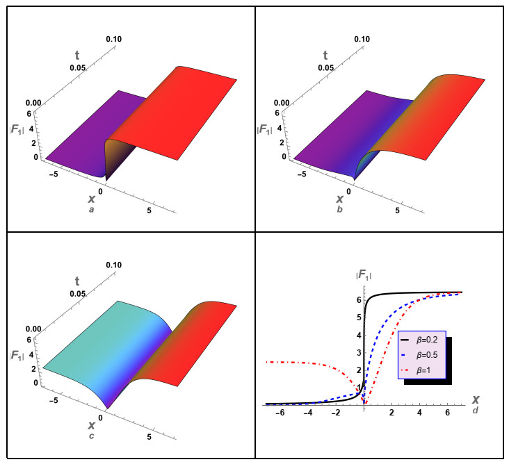
Figure 1. The solution

$\vert$

$F_{1}(x, t)|$ is plotted against the space-fractional parameter

$\beta$ : (a) 3D graphic for the solution given by Eq (3.7) at

$\beta = 0.2$ , (b) 3D graphic for the solution given by Eq (3.7) at

$\beta = 0.5$ , (c) 3D graphic for the solution given by Eq (3.7) at

$\beta = 1$ , (d) 2D graphic for the solution given by Eq (3.7) at different values of

$\beta$ . Here,

$\alpha = 1$ ,

$\lambda = 5$ ,

$\mu = \sqrt{-2}$ ,

$\chi = 2$ ,

$A = 1$ , and

$B = 1$ .

DownLoad: Full-Size Img PowerPoint

Figure 2. The solution

$\vert$

$F_{1}(x, t)|$ is plotted against the time-fractional parameter

$\alpha$ : (a) 3D graphic for the solution given by Eq (3.7) at

$\alpha = 0.2$ , (b) 3D graphic for the solution given by Eq (3.7) at

$\alpha = 0.4$ , (c) 3D graphic for the solution given by Eq (3.7) at

$\alpha = 1$ , (d) 2D graphic for the solution given by Eq (3.7) at different values of

$\alpha$ . Here,

$\beta = 1$ ,

$\lambda = 5$ ,

$\mu = \sqrt{-2}$ ,

$\chi = 2$ ,

$A = 1$ , and

$B = 1$ .

DownLoad: Full-Size Img PowerPoint

Figure 3. The solution

$\vert$

$F_{2}(x, t)|$ is plotted against the space-fractional parameter

$\beta$ : (a) 3D graphic for the solution given by Eq (3.8) at

$\beta = 0.1$ , (b) 3D graphic for the solution given by Eq (3.8) at

$\beta = 0.2$ , (c) 3D graphic for the solution given by Eq (3.8) at

$\beta = 0.3$ , (d) 2D graphic for the solution given by Eq (3.8) at different values of

$\beta$ . Here,

$\alpha = 1$ ,

$\lambda = 5$ ,

$\mu = \sqrt{-2}$ ,

$\chi = 2$ ,

$A = 0.1$ , and

$B = 10$ .

DownLoad: Full-Size Img PowerPoint

Figure 4. The solution

$\vert$

$F_{2}(x, t)|$ is plotted against the time-fractional parameter

$\alpha$ : (a) 3D graphic for the solution given by Eq (3.8) at

$\alpha = 0.2$ , (b) 3D graphic for the solution given by Eq (3.8) at

$\alpha = 0.4$ , (c) 3D graphic for the solution given by Eq (3.8) at

$\alpha = 1$ , (d) 2D graphic for the solution given by Eq (3.8) at different values of

$\alpha$ . Here,

$\beta = 1$ ,

$\lambda = 5$ ,

$\mu = \sqrt{-2}$ ,

$\chi = 2$ ,

$A = 0.1$ , and

$B = 10$ .

DownLoad: Full-Size Img PowerPoint

Figure 5. The solution

$\vert$

$F_{3}(x, t)|$ is plotted against the space-fractional parameter

$\beta$ : (a) 3D graphic for the solution given by Eq (3.9) at

$\beta = 0.2$ , (b) 3D graphic for the solution given by Eq (3.9) at

$\beta = 0.4$ , (c) 3D graphic for the solution given by Eq (3.9) at

$\beta = 0.7$ , (d) 2D graphic for the solution given by Eq (3.9) at different values of

$\beta$ . Here,

$\alpha = 1$ ,

$\lambda = 2$ ,

$\mu = 10$ ,

$\chi = 2$ ,

$A = 1$ , and

$B = 1$ .

DownLoad: Full-Size Img PowerPoint

Figure 6. The solution

$\vert$

$F_{3}(x, t)|$ is plotted against the time-fractional parameter

$\alpha$ : (a) 3D graphic for the solution given by Eq (3.9) at

$\alpha = 0.2$ , (b) 3D graphic for the solution given by Eq (3.9) at

$\alpha = 0.4$ , (c) 3D graphic for the solution given by Eq (3.9) at

$\alpha = 0.7$ , (d) 2D graphic for the solution given by Eq (3.9) at different values of

$\alpha$ . Here,

$\beta = 1$ ,

$\lambda = 2$ ,

$\mu = 10$ ,

$\chi = 2$ ,

$A = 1$ , and

$B = 1$ .

DownLoad: Full-Size Img PowerPoint

Figure 7. The solution

$\vert$

$F_{4}(x, t)|$ is plotted against the space-fractional parameter

$\beta$ : (a) 3D graphic for the solution given by Eq (3.10) at

$\beta = 0.2$ , (b) 3D graphic for the solution given by Eq (3.10) at

$\beta = 0.4$ , (c) 3D graphic for the solution given by Eq (3.10) at

$\beta = 0.7$ , (d) 2D graphic for the solution given by Eq (3.10) at different values of

$\beta$ . Here,

$\alpha = 1$ ,

$\lambda = 2$ ,

$\mu = 10$ ,

$\chi = 2$ ,

$A = 0.1$ , and

$B = 10$ .

DownLoad: Full-Size Img PowerPoint

Figure 8. The solution

$\vert$

$F_{4}(x, t)|$ is plotted against the time-fractional parameter

$\alpha$ : (a) 3D graphic for the solution given by Eq (3.10) at

$\alpha = 0.2$ , (b) 3D graphic for the solution given by Eq (3.10) at

$\alpha = 0.4$ , (c) 3D graphic for the solution given by Eq (3.10) at

$\alpha = 0.7$ , (d) 2D graphic for the solution given by Eq (3.10) at different values of

$\alpha$ . Here,

$\beta = 1$ ,

$\lambda = 2$ ,

$\mu = 10$ ,

$\chi = 2$ ,

$A = 0.1$ , and

$B = 10$ .

DownLoad: Full-Size Img PowerPoint

Figure 9. The solution

$\vert$

$F_{5}(x, t)|$ is plotted against the space-fractional parameter

$\beta$ : (a) 3D graphic for the solution given by Eq (3.11) at

$\beta = 0.2$ , (b) 3D graphic for the solution given by Eq (3.11) at

$\beta = 0.4$ , (c) 3D graphic for the solution given by Eq (3.11) at

$\beta = 0.7$ , (d) 2D graphic for the solution given by Eq (3.11) at different values of

$\beta$ . Here,

$\alpha = 1$ ,

$\lambda = -2$ ,

$\mu = -2$ ,

$\chi = 10$ ,

$A = 0.1$ , and

$B = 10$ .

DownLoad: Full-Size Img PowerPoint

Figure 10. The solution

$\vert$

$F_{5}(x, t)|$ is plotted against the time-fractional parameter

$\alpha$ : (a) 3D graphic for the solution given by Eq (3.11) at

$\alpha = 0.2$ , (b) 3D graphic for the solution given by Eq (3.11) at

$\alpha = 0.4$ , (c) 3D graphic for the solution given by Eq (3.11) at

$\alpha = 0.7$ , (d) 2D graphic for the solution given by Eq (3.11) at different values of

$\alpha$ . Here,

$\beta = 1$ ,

$\lambda = -2$ ,

$\mu = -2$ ,

$\chi = 10$ ,

$A = 0.1$ , and

$B = 10$ .

DownLoad: Full-Size Img PowerPoint

We analyzed all of the derived solutions graphically, as shown in Figures 1–10, by using some random values for the associated parameters and coefficients of the equation. The absolute value of the solution given by Eq (3.7) was examined as elucidated in and , which was evaluated against the space- and time-fractional parameters $\beta$ and $\alpha$ , respectively. As shown in , increasing the space-fractional parameter turns the shock wave into a quasi-peakon wave. The impact of the time-fractional parameter on the characteristics of the quasi-peakon wave is illustrated in . Furthermore, an investigation was conducted to examine the impact of space- and time fractional parameters $\beta$ and $\alpha$ on the profile of the solution given by Eq (3.8), as depicted in Figures 3 and , respectively. Based on the data presented in , it can be observed that for $\alpha = 1$ , when the space-fractional parameter $\beta$ is altered, the solution's form remains consistent with the shock wave's shape. However, as $\beta$ increases, the shock wave amplitude decreases. further illustrates the impact of the time-fractional parameter $\alpha$ on the visual representation of the solution given by Eq (3.8), which exhibits characteristics akin to a peakon waveform. The solutions given by Eqs(3.9) and (3.10) for the case that $\tau > 0$ are also examined, as depicted in Figures 5–8. and display the shock-like solution given by Eq (3.9) against both the space- and time-fractional parameters $\beta$ and $\alpha$ , respectively. Additionally, we analyzed the influence of both the space- and time-fractional parameters $\beta$ and $\alpha$ on the characteristics of the solution given by Eq (3.10), as depicted in and , correspondingly. Ultimately, we conducted a graphical analysis of the quasi-peakon wave solution given by Eq (3.11) and examined the impact of both the space- and time-fractional parameters $\beta$ and $\alpha$ on its behavior, as depicted in Figures 9 and 10, respectively.

5. Conclusion

The fractional DGH equation has been analytically solved by using the Riccati-Bernoulli sub-optimal differential equation method together with the Bäcklund transformation. We correctly obtained several travelling wave solutions in the form of hyperbolic, periodic, and rational solutions by applying the given norm; yielding a hierarchy of traveling wave solutions, including the quasi-peakon wave, shock-like wave, compacton-like wave, and other periodic waves. The resultant solutions were subjected to numerical analysis, wherein some random values were assigned to the related coefficients and parameters. The effects of both space- and time-fractional parameters on the properties and behavior of all derived solutions was also examined. It has been found that the behavior of the derived solutions is significantly influenced by changing the values of both the space- and time-fractional parameters. By altering these parameters we found that, they not only affect the amplitude and width of the waves described by these solutions they also impact the transition between the waves. This finding represents a crucial outcome of our research. The obtained results demonstrate that the employed techniques are a direct and effective strategy for addressing highly complicated and strong nonlinear evolution/wave equations. They yield a substantial number of analytical solutions, which can help many researchers interpret their distinct results.

It is essential to acknowledge that the numerical analysis of the acquired results and the graphical representation of the derived solutions were conducted by using Wolfram MATHEMATICA 13.2.

Future work: The results indicate that the current technique offers many analytical solutions, allowing researchers to utilize this approach to simulate various physical and engineering problems. Thus, this approach is expected to efficiently examine and simulate a range of evolution/wave equations that describe various nonlinear phenomena in different plasma models. One example of its use is the analysis of the space-time fractional KdV-type equations ^[52,53] and the space-time fractional Kawahara-type equations ^[54,55,56], which allows for an examination of the impact of fractional parameters on the generated solutions' profiles. Therefore, it is possible to study the effects of fractional coefficients on the behavior of the nonlinear structures described by these families of KdV-type and Kawahara-type equations, such as solitary waves, shock waves, cnoidal waves, and periodic waves. Furthermore, this method can be applied to examine nonlinear Schrödinger-type equations to investigate the impact of fractional parameters on the characteristics of envelope-modulated waves, such as bright and dark envelope solitons, rogue waves, and breathers, and modulated cnoidal waves ^[57,58]. Therefore, this method is expected to have promising, effective, and fertile results in that can help to explain many mysterious nonlinear phenomena that arise and propagate in various plasma models.

Author contributions

Humaira Yasmin, Haifa A. Alyousef, Sadia Asad, Imran Khan, R. T. Matoog, S. A. El-Tantawy: writing, review, editing, and visualization. All authors of this article have been contributed equally. All authors have read and approved the final version of the manuscript for publication.

Use of AI tools declaration

The authors declare that they have not used Artificial Intelligence tools in the creation of this article.

Acknowledgments

The authors express their gratitude to Princess Nourah bint Abdulrahman University Researchers Supporting Project Number (PNURSP2024R17), Princess Nourah bint Abdulrahman University, Riyadh, Saudi Arabia. This work was supported by the Deanship of Scientific Research, Vice Presidency for Graduate Studies and Scientific Research, King Faisal University, Saudi Arabia (GrantA152).

Funding

Conflict of interest

The authors declare that they have no conflicts of interest.

References

[1]	M. Caputo, Linear model of dissipation whose Q is almost frequency independent-Ⅱ, Geophys. J. R. Astron. Soc., 13 (1967), 529–539. https://doi.org/10.1111/j.1365-246X.1967.tb02303.x doi: 10.1111/j.1365-246X.1967.tb02303.x
[2]	I. Podlubny, Fractional Differential Equations: An Introduction to Fractional Derivatives, Fractional Differential Equations, to Methods of Their Solution and Some of Their Applications, Elsevier, 1998.
[3]	M. Caputo, M. Fabrizio, A new definition of fractional derivative without singular kernel, Progr. Fract. Differ. Appl., 1 (2015), 73–85. http://dx.doi.org/10.12785/pfda/010201 doi: 10.12785/pfda/010201
[4]	A. Atangana, D. Baleanu, New fractional derivatives with non-local and non-singular kernel: Theory and application to heat transfer model, Therm. Sci., 20 (2016), 763–769. https://doi.org/10.2298/TSCI160111018A doi: 10.2298/TSCI160111018A
[5]	W. Chen, Time-space fabric underlying anomalous diffusion, Chaos, Solitons Fractals, 28 (2006), 923–929. https://doi.org/10.1016/j.chaos.2005.08.199 doi: 10.1016/j.chaos.2005.08.199
[6]	A. Atangana, Fractal-fractional differentiation and integration: Connecting fractal calculus and fractional calculus to predict complex system, Chaos, Solitons Fractals, 102 (2017), 396–406. https://doi.org/10.1016/j.chaos.2017.04.027 doi: 10.1016/j.chaos.2017.04.027
[7]	J. He, X. Zhang, L. Liu, Y. Wu, Y. Cui, Existence and asymptotic analysis of positive solutions for a singular fractional differential equation with nonlocal boundary conditions, Boundary Value Probl., 2018 (2018). https://doi.org/10.1186/s13661-018-1109-5
[8]	J. Wu, X. Zhang, L. Liu, Y. Wu, Y. Cui, Convergence analysis of iterative scheme and error estimation of positive solution for a fractional differential equation, Math. Model. Anal., 23 (2018), 611–626. https://doi.org/10.3846/mma.2018.037 doi: 10.3846/mma.2018.037
[9]	X. Zhang, L. Liu, Y. Wu, Y. Cui, New result on the critical exponent for solution of an ordinary fractional differential problem, J. Funct. Spaces, 2017 (2017), 3976469. https://doi.org/10.1155/2017/3976469 doi: 10.1155/2017/3976469
[10]	G. D. Li, Y. Zhang, Y. J. Guan, W. J. Li, Stability analysis of multi-point boundary conditions for fractional differential equation with non-instantaneous integral impulse, Math. Biosci. Eng., 20 (2023), 7020–7041. https://doi.org/10.3934/mbe.2023303 doi: 10.3934/mbe.2023303
[11]	D. Luo, M. Tian, Q. Zhu, Some results on finite-time stability of stochastic fractional-order delay differential equations, Chaos, Solitons Fractals, 158 (2022). https://doi.org/10.1016/j.chaos.2022.111996
[12]	Y. Zhao, L. Wang, Practical exponential stability of impulsive stochastic food chain system with time-varying delays, Mathematics, 11 (2023), 147. https://doi.org/10.3390/math11010147 doi: 10.3390/math11010147
[13]	M. Xia, L. Liu, J. Fang, Y. Zhang, Stability analysis for a class of stochastic differential equations with impulses, Mathematics, 11 (2023), 1541. https://doi.org/10.3390/math11061541 doi: 10.3390/math11061541
[14]	B. Wang, Q. Zhu, Stability analysis of discrete-time semi-Markov jump linearsystems with time delay, IEEE Trans. Autom., 68 (2023), 6758–6765. https://doi.org/10.1109/TAC.2023.3240926 doi: 10.1109/TAC.2023.3240926
[15]	Q. Zhu, Stabilization of stochastic nonlinear delay systems with exogenousdisturbances and the event-triggered feedback control, IEEE Trans. Autom., 64 (2019), 3764–3771. https://doi.org/10.1109/TAC.2018.2882067 doi: 10.1109/TAC.2018.2882067
[16]	A. Atangana, S. I. Araz, New concept in calculus: Piecewise differential and integral operators, Chaos, Solitons Fractals, 145 (2021). https://doi.org/10.1016/j.chaos.2020.110638
[17]	A. Atangana, S. I. Araz, A modified parametrized method for ordinary differential equations with nonlocal operators, HAL, 2022.
[18]	C. Liping, M. A. Khan, A. Atangana, S. Kumar, A new financial chaotic model in Atangana-Baleanu stochastic fractional differential equations, Alex. Eng. J., 60 (2021), 5193–5204. https://doi.org/10.1016/j.aej.2021.04.023 doi: 10.1016/j.aej.2021.04.023
[19]	C. Carathéodory, Über den Variabilitätsbereich der Koeffizienten von Potenzreihen, die gegebene Werte nicht annehmen, Math. Ann., 64 (1907), 95–115. https://doi.org/10.1007/BF01449883 doi: 10.1007/BF01449883
[20]	A. Atangana, S. I. Araz, Theory and methods of piecewise defined fractional operators, Elsevier, in press.
[21]	W. Wang, S. Cheng, Z. Guo, X. Yan, A note on the continuity for Caputo fractional stochastic differential equations, Chaos, 30 (2020), 073106. https://doi.org/10.1063/1.5141485 doi: 10.1063/1.5141485
[22]	A. Ahmadova, N. I. Mamudov, Existence and uniqueness results for a class of fractional stochastic neutral differential equations, Chaos, Solitons Fractals, 139 (2020), 110253. https://doi.org/10.1016/j.chaos.2020.110253 doi: 10.1016/j.chaos.2020.110253
[23]	A. Atangana, S. I. Araz, Step forward on nonlinear differential equations with the Atangana-Baleanu derivative: Inequalities, existence, uniqueness and method, Chaos, Solitons Fractals, 173 (2023), 113700. https://doi.org/10.1016/j.chaos.2023.113700 doi: 10.1016/j.chaos.2023.113700
[24]	D. F. Griffiths, D. J. Higham, Numerical Methods for Ordinary Differential Equations: Initial Value Problems, Springer Undergraduate Mathematics Series, Springer, 2010.
[25]	E. Süli, D. F. Mayers, An Introduction to Numerical Analysis, Cambridge University Press, 2003. https://doi.org/10.1017/CBO9780511801181
[26]	J. C. Butcher, Numerical Methods for Ordinary Differential Equations, John Wiley, 2023.
[27]	T. Mekkaoui, A. Atangana, S. I. Araz, Predictor-corrector for non-linear differential and integral equation with fractal-fractional operators, Eng. Comput., 37 (2020), 2359–2368. https://doi.org/10.1007/s00366-020-00948-6 doi: 10.1007/s00366-020-00948-6
[28]	S. W. Teklu, Analysis of fractional order model on higher institution students' anxiety towards mathematics with optimal control theory, Sci. Rep., 13 (2023), 6867. https://doi.org/10.1038/s41598-023-33961-y doi: 10.1038/s41598-023-33961-y
[29]	D. A. Getahun, G. Adamu, A. Andargie, J. D. Mebrat, Predicting mathematics performance from anxiety, enjoyment, value, and self-efficacy beliefs towards mathematics among engineering majors, Bahir Dar J. Educ., 16 (2016).
[30]	A. Atangana, S. I. Araz, A successive midpoint method for nonlinear differential equations with classical and Caputo-Fabrizio derivatives, AIMS Math., 8 (2023), 27309–27327. https://doi.org/10.3934/math.20231397 doi: 10.3934/math.20231397
[31]	A. Akin, I. N. Kurbanoglu, The relationships between math anxiety, math attitudes, and self-efficacy: A structural equation model, Stud. Psychol., 53 (2011), 263.

This article has been cited by:

1.	Bálint Máté Takács, Gabriella Svantnerné Sebestyén, István Faragó, High-order reliable numerical methods for epidemic models with non-constant recruitment rate, 2024, 206, 01689274, 75, 10.1016/j.apnum.2024.08.008
2.	Bruno Buonomo, Eleonora Messina, Claudia Panico, Antonia Vecchio, An integral renewal equation approach to behavioural epidemic models with information index, 2025, 90, 0303-6812, 10.1007/s00285-024-02172-y

Reader Comments

Your name:*

Email:*
© 2024 the Author(s), licensee AIMS Press. This is an open access article distributed under the terms of the Creative Commons Attribution License (http://creativecommons.org/licenses/by/4.0)

通讯作者: 陈斌, bchen63@163.com

1.
沈阳化工大学材料科学与工程学院沈阳 110142

Electronic Research Archive

1.1 1.7

Metrics

Article views(1634) PDF downloads(118) Cited by(2)

Preview PDF

Download XML

Export Citation

Article outline

Show full outline

Electronic Research Archive

Existence, uniqueness and numerical solution of stochastic fractional differential equations with integer and non-integer orders

Related Papers:

Abstract

1. Introduction

2. Methodology

3. Execution of the problem

4. Results and discussion

5. Conclusion

Author contributions

Use of AI tools declaration

Acknowledgments

Funding

Conflict of interest

References

This article has been cited by:

Reader Comments

通讯作者: 陈斌, bchen63@163.com

Metrics

Figures and Tables

Other Articles By Authors

Catalog

Abstract

1. Introduction

2. Methodology

3. Execution of the problem

4. Results and discussion

5. Conclusion

Author contributions

Use of AI tools declaration

Acknowledgments

Funding

Conflict of interest

References

Electronic Research Archive

Existence, uniqueness and numerical solution of stochastic fractional differential equations with integer and non-integer orders

Related Papers:

Abstract

1. Introduction

2. Methodology

3. Execution of the problem

4. Results and discussion

5. Conclusion

Author contributions

Use of AI tools declaration

Acknowledgments

Funding

Conflict of interest

References

This article has been cited by:

Reader Comments

通讯作者: 陈斌, bchen63@163.com

Metrics

Figures and Tables

Other Articles By Authors

Related pages

Tools

Export File

Citation

Format

Content

Catalog

Abstract

1. Introduction

2. Methodology

3. Execution of the problem

4. Results and discussion

5. Conclusion

Author contributions

Use of AI tools declaration

Acknowledgments

Funding

Conflict of interest

References