Straddle monorail noise impact evaluation considering acoustic propagation characteristics and the subjective feelings of residents

J. S. Peng; Q. W. Kong; Y. X. Gao; L. Zhang; J. S. Peng; Q. W. Kong; Y. X. Gao; L. Zhang

doi:10.3934/era.2023370

Electronic Research Archive

2023, Volume 31, Issue 12: 7307-7336. doi: 10.3934/era.2023370

Previous Article Next Article

Research article Special Issues

Straddle monorail noise impact evaluation considering acoustic propagation characteristics and the subjective feelings of residents

1.
School of Traffic & Transportation, Chongqing Jiaotong University, Chongqing 400074, China
2.
School of Mechanical and Traffic Engineering, Ordos Institute of Technology, Ordos 017000, China

Received: 19 July 2023 Revised: 25 October 2023 Accepted: 30 October 2023 Published: 14 November 2023

In this study, a novel method of evaluating the impact of straddle monorail noise on residential areas considering both objective and subjective effects was developed, in view of the singleness of the existing evaluation method of the track noise impact on residential areas. Using a questionnaire, the quantified straddle monorail noise data for five typical apartment complexes with rail-side layouts were combined with data on the subjective feelings of residents regarding this noise. Then, a model for evaluating the impact of the straddle monorail noise on residential areas under subjective and objective conditions was constructed. Finally, by considering the impacts of straddle monorail noise in residential areas, prevention and control measures were proposed that targeted the acoustic source, sound propagation process, and receiving location. The proposed evaluation method, which considered the needs of residents, could be used to improve straddle monorail noise impact evaluation systems and provide a scientific reference for improving acoustic environments in residential areas along straddle monorail lines.
- straddle monorail noise,
- residential area,
- noise measurement,
- subjective feeling,
- comprehensive evaluation
Citation: J. S. Peng, Q. W. Kong, Y. X. Gao, L. Zhang. Straddle monorail noise impact evaluation considering acoustic propagation characteristics and the subjective feelings of residents[J]. Electronic Research Archive, 2023, 31(12): 7307-7336. doi: 10.3934/era.2023370

Related Papers:

Abstract

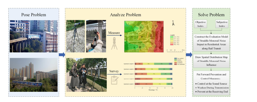
In this study, a novel method of evaluating the impact of straddle monorail noise on residential areas considering both objective and subjective effects was developed, in view of the singleness of the existing evaluation method of the track noise impact on residential areas. Using a questionnaire, the quantified straddle monorail noise data for five typical apartment complexes with rail-side layouts were combined with data on the subjective feelings of residents regarding this noise. Then, a model for evaluating the impact of the straddle monorail noise on residential areas under subjective and objective conditions was constructed. Finally, by considering the impacts of straddle monorail noise in residential areas, prevention and control measures were proposed that targeted the acoustic source, sound propagation process, and receiving location. The proposed evaluation method, which considered the needs of residents, could be used to improve straddle monorail noise impact evaluation systems and provide a scientific reference for improving acoustic environments in residential areas along straddle monorail lines.

References

[1]	Z. Y. Tao, Y. M. Wang, M. Sanaye, J. A. Moore, C. Zou, Experimental study of train-induced vibration in over-track buildings in a metro depot, Eng. Struct., 198 (2019), 109473. https://doi.org/10.1016/j.engstruct.2019.109473 doi: 10.1016/j.engstruct.2019.109473
[2]	Z. Y. Tao, J. A. Moore, M. Sanaye, Y. M. Wang, C. Zou, Train-induced floor vibration and structure-borne noise predictions in a low-rise over-track building, Eng. Struct., 255 (2022), 113914. https://doi.org/10.1016/j.engstruct.2022.113914 doi: 10.1016/j.engstruct.2022.113914
[3]	C. Zou, Y. M. Wang, P. Wang, J. X. Guo, Measurement of ground and nearby building vibration and noise induced by trains in a metro depot, Sci. Total Environ., 536 (2015), 761–773. https://doi.org/10.1016/j.scitotenv.2015.07.123 doi: 10.1016/j.scitotenv.2015.07.123
[4]	C. Zou, Y. M. Wang, J. A. Moore, M. Sanayei, Train-induced field vibration measurements of ground and over-track buildings, Sci. Total Environ., 575 (2017), 1339–1351. https://doi.org/10.1016/j.scitotenv.2016.09.216 doi: 10.1016/j.scitotenv.2016.09.216
[5]	P. Tassi, O. Rohmer, S. Schimchowitsch, A. Eschenlauer, A. Bonnefond, F. Margiocchi, et al., Living alongside railway tracks: Long-term effects of nocturnal noise on sleep and cardiovascular reactivity as a function of age, Environ. Int., 36 (2010), 683–689. https://doi.org/10.1016/j.envint.2010.05.001 doi: 10.1016/j.envint.2010.05.001
[6]	D. Petri, G. Licitra, M. A. Vigotti, L. Fredianelli, Effects of exposure to road, railway, airport and recreational noise on blood pressure and hypertension, Int. J. Environ. Res. Public Health, 18 (2021), 9145. https://doi.org/10.3390/ijerph18179145 doi: 10.3390/ijerph18179145
[7]	S. Sanok, M. Berger, U. Müller, M. Schmid, S. Weidenfeld, E. M. Elmenhorst, et al., Road traffic noise impacts sleep continuity in suburban residents: Exposure-response quantification of noise-induced awakenings from vehicle pass-bys at night, Sci. Total Environ., 817 (2022), 152594. https://doi.org/10.1016/j.scitotenv.2021.152594 doi: 10.1016/j.scitotenv.2021.152594
[8]	M. Shamsipour, N. Zaredar, M. R. Monazzam, Z. Namvar, S. Mohammadpour, Burden of diseases attributed to traffic noise in the metropolis of Tehran in 2017, Environ. Pollut., 301 (2022), 119042. https://doi.org/10.1016/j.envpol.2022.119042 doi: 10.1016/j.envpol.2022.119042
[9]	R. Rylander, Physiological aspects of noise-induced stress and annoyance, J. Sound Vib., 277 (2004), 471–478. https://doi.org/10.1016/j.jsv.2004.03.008 doi: 10.1016/j.jsv.2004.03.008
[10]	G. Jigeer, W. M. Tao, Q. Q. Zhu, X. Y. Xu, Y. Zhao, H. D. Kan, et al., Association of residential noise exposure with maternal anxiety and depression in late pregnancy, Environ. Int., 168 (2022), 107473. https://doi.org/10.1016/j.envint.2022.107473 doi: 10.1016/j.envint.2022.107473
[11]	N. Roswall, O. Raaschou-Nielsen, S. S. Jensen, A. Tjønneland, M. Sørensen, Long-term exposure to residential railway and road traffic noise and risk for diabetes in a Danish cohort, Environ. Res., 160 (2018), 292–297. https://doi.org/10.1016/j.envres.2017.10.008 doi: 10.1016/j.envres.2017.10.008
[12]	M. Foraster, I. C. Eze, D. Vienneau, E. Schaffner, A. Jeong, H. Héritier, et al., Long-term exposure to transportation noise and its association with adiposity markers and development of obesity, Environ. Int., 121 (2018), 879–889. https://doi.org/10.1016/j.envint.2018.09.057 doi: 10.1016/j.envint.2018.09.057
[13]	Y. T. Cai, W. L. Zijlema, E. P. Sørgjerd, D. Doiron, K. D. Hoogh, S. Hodgson, et al., Impact of road traffic noise on obesity measures: Observational study of three European cohorts, Environ. Res., 191 (2020), 110013. https://doi.org/10.1016/j.envres.2020.110013 doi: 10.1016/j.envres.2020.110013
[14]	M. Sørensen, P. Lühdorf, M. Ketzel, Z. J. Andersen, A. Tjønneland, K. Overvad, et al., Combined effects of road traffic noise and ambient air pollution in relation to risk for stroke?, Environ. Res., 133 (2014), 49–55. https://doi.org/10.1016/j.envres.2014.05.011 doi: 10.1016/j.envres.2014.05.011
[15]	A. Pyko, N. Andersson, C. Eriksson, U. D. Faire, T. Lind, N. Mitkovskaya, et al., Long-term transportation noise exposure and incidence of ischaemic heart disease and stroke: a cohort study, Occup. Environ. Med., 76 (2019), 201–207. https://doi.org/10.1097/01.EE9.0000609496.01738.ac doi: 10.1097/01.EE9.0000609496.01738.ac
[16]	J. Weuve, J. D'Souza, T. Beck, D. A. Evans, J. D. Kaufman, K. B. Rajan, et al., Long‐term community noise exposure in relation to dementia, cognition, and cognitive decline in older adults, Alzheimer's Dementia, 17 (2021), 525–533. https://doi.org/10.1002/alz.12191 doi: 10.1002/alz.12191
[17]	C. B. Cai, Q. L. He, S. Y. Zhu, W. M. Zhai, M. Z. Wang, Dynamic interaction of suspension-type monorail vehicle and bridge: Numerical simulation and experiment, Mech. Syst. Signal Process., 118 (2019), 388–407. https://doi.org/10.1016/j.ymssp.2018.08.062 doi: 10.1016/j.ymssp.2018.08.062
[18]	F. Q. Guo, K. Y. Chen, F. G. Gu, H. Wang, T. Wen, Reviews on current situation and development of straddle-type monorail tour transit system in China, J. Cent. South Univ. (Sci. Technol.), 52 (2021), 4540–4551. https://doi.org/10.11817/j.issn.1672-7207.2021.12.034 doi: 10.11817/j.issn.1672-7207.2021.12.034
[19]	F. Bunn, P. H. T. Zannin, Assessment of railway noise in an urban setting, Appl. Acoust., 104 (2016), 16–23. https://doi.org/10.1016/j.apacoust.2015.10.025 doi: 10.1016/j.apacoust.2015.10.025
[20]	W. J. Yang, J. Y. He, C. M. He, M. Cai, Evaluation of urban traffic noise pollution based on noise maps, Transp. Res. Part D Transp. Environ., 87 (2020), 102516. https://doi.org/10.1016/j.trd.2020.102516 doi: 10.1016/j.trd.2020.102516
[21]	A. Tombolato, F. Bonomini, A. D. Bella, Methodology for the evaluation of low-frequency environmental noise: a case-study, Appl. Acoust., 187 (2022), 108517. https://doi.org/10.1016/j.apacoust.2021.108517 doi: 10.1016/j.apacoust.2021.108517
[22]	L. P. S. Fernández, Environmental noise indicators and acoustic indexes based on fuzzy modelling for urban spaces, Ecol. Indic., 126 (2021), 107631. https://doi.org/10.1016/j.ecolind.2021.107631 doi: 10.1016/j.ecolind.2021.107631
[23]	R. H. Liang, W. F. Liu, W. B. Li, Z. Z. Wu, A traffic noise source identification method for buildings adjacent to multiple transport infrastructures based on deep learning, Build. Environ., 211 (2022), 108764. https://doi.org/10.1016/j.buildenv.2022.108764 doi: 10.1016/j.buildenv.2022.108764
[24]	H. Di, X. P. Liu, J. Q. Zhang, Z. J. Tong, M. C. Ji, F. X. Li, et al., Estimation of the quality of an urban acoustic environment based on traffic noise evaluation models, Appl. Acoust., 141 (2018), 115–124. https://doi.org/10.1016/j.apacoust.2018.07.010 doi: 10.1016/j.apacoust.2018.07.010
[25]	T. Y. Chang, C. H. Liang, C. F. Wu, L. T. Chang, Application of land-use regression models to estimate sound pressure levels and frequency components of road traffic noise in Taichung, Taiwan, Environ. Int., 131 (2019), 104959. https://doi.org/10.1016/j.envint.2019.104959 doi: 10.1016/j.envint.2019.104959
[26]	H. B. Wang, Z. Y. Wu, J. C. Chen, L. Chen, Evaluation of road traffic noise exposure considering differential crowd characteristics, Transp. Res. Part D Transp. Environ., 105 (2022), 103250. https://doi.org/10.1016/j.trd.2022.103250 doi: 10.1016/j.trd.2022.103250
[27]	T. Morihara, S. Yokoshima, Y. Matsumoto, Effects of noise and vibration due to the Hokuriku Shinkansen railway on the living environment: A socio-acoustic survey one year after the opening, Int. J. Environ. Res. Public Health, 18 (2021), 7794. https://doi.org/10.3390/ijerph18157794 doi: 10.3390/ijerph18157794
[28]	L. Zhang, H. Ma, Investigation of Chinese residents' community response to high-speed railway noise, Appl. Acoust., 172 (2021), 107615. https://doi.org/10.1016/j.apacoust.2020.107615 doi: 10.1016/j.apacoust.2020.107615
[29]	D. S. Michaud, L. Marro, A. Denning, S. Shackleton, N. Toutant, J. P. McNamee, Annoyance toward transportation and construction noise in rural suburban and urban regions across Canada, Environ. Impact Assess. Rev., 97 (2022), 106881. https://doi.org/10.1016/j.eiar.2022.106881 doi: 10.1016/j.eiar.2022.106881
[30]	G. Licitra, L. Fredianelli, D. Petri, M. A. Vigotti, Annoyance evaluation due to overall railway noise and vibration in Pisa urban areas, Sci. Total Environ., 568 (2016), 1315–1325. https://doi.org/10.1016/j.scitotenv.2015.11.071 doi: 10.1016/j.scitotenv.2015.11.071
[31]	H. Xie, H. Li, C. Liu, M. Y. Li, J. W. Zou, Noise exposure of residential areas along LRT lines in a mountainous city, Sci. Total Environ., 568 (2016), 1283–1294. https://doi.org/10.1016/j.scitotenv.2016.03.097 doi: 10.1016/j.scitotenv.2016.03.097
[32]	Environmental Quality Standard for Noise, China Environment Science Press, 2008, GB 3096-2008.
[33]	Technical Guidelines for Environmental Impact Assessment—Urban Rail Transit, Ministry of Ecology and Environment of the People's Republic of China, (2018), HJ 453-2018.
[34]	L. Li, T. F. Yin, Q. Zhu, Y. Y. Luo, Characteristics and energies in different frequency bands of environmental noise in urban elevated rail, J. Traffic Transp. Eng., 18 (2018), 120–128. https://doi.org/10.19818/j.cnki.1671-1637.2018.02.013 doi: 10.19818/j.cnki.1671-1637.2018.02.013
[35]	U. Landström, E. Åkerlund, A. Kjellberg, M. Tesarz, Exposure levels, tonal components, and noise annoyance in working environments, Environ. Int., 21 (1995), 265–275. https://doi.org/10.1016/0160-4120(95)00017-F doi: 10.1016/0160-4120(95)00017-F
[36]	T. Alvares-Sanches, P. E. Osborne, P. R. White, Mobile surveys and machine learning can improve urban noise mapping: Beyond A-weighted measurements of exposure, Sci. Total Environ., 775 (2021), 145600. https://doi.org/10.1016/j.scitotenv.2021.145600 doi: 10.1016/j.scitotenv.2021.145600
[37]	M. Lefèvre, A. Chaumond, P. Champelovier, L. G. Allemand, J. Lambert, B. Laumon, et al., Understanding the relationship between air traffic noise exposure and annoyance in populations living near airports in France, Environ. Int., 144 (2020), 106058. https://doi.org/10.1016/j.envint.2020.106058 doi: 10.1016/j.envint.2020.106058
[38]	W. J. Yin, Z. F. Ming, Electric vehicle charging and discharging scheduling strategy based on local search and competitive learning particle swarm optimization algorithm, J. Energy Storage, 42 (2021), 102966. https://doi.org/10.1016/j.est.2021.102966 doi: 10.1016/j.est.2021.102966
[39]	T. L. Saaty, L. G. Vargas, The seven pillars of the analytic hierarchy process, in Models, Methods, Concepts & Applications of the Analytic Hierarchy Process, Springer US, Boston, MA, 175 (2012), 23–40. https://doi.org/10.1007/978-1-4614-3597-6_2
[40]	J. A. Alves, F. N. Paiva, L. T. Silva, P. Remoaldo, Low-frequency noise and its main effects on human health—A review of the literature between 2016 and 2019, Appl. Sci., 10 (2020), 5205. https://doi.org/10.3390/app10155205 doi: 10.3390/app10155205
[41]	Y. Inukai, H. Taya, S. Yamada, Thresholds and acceptability of low frequency pure tones by sufferers, J. Low Freq. Noise Vibr. Act. Control, 24 (2005), 163–169. https://doi.org/10.1260/026309205775374433 doi: 10.1260/026309205775374433
[42]	E. Murphy, E. A. King, An assessment of residential exposure to environmental noise at a shipping port, Environ. Int., 63 (2014), 207–215. https://doi.org/10.1016/j.envint.2013.11.001 doi: 10.1016/j.envint.2013.11.001
[43]	B. Schäffer, M. Brink, F. Schlatter, D. Vienneau, J. M. Wunderli, Residential green is associated with reduced annoyance to road traffic and railway noise but increased annoyance to aircraft noise exposure, Environ. Int., 143 (2020), 105885. https://doi.org/10.1016/j.envint.2020.105885 doi: 10.1016/j.envint.2020.105885
[44]	K. Vogiatzis, P. Vanhonacker, Noise reduction in urban LRT networks by combining track based solutions, Sci. Total Environ., 68 (2016), 1344–1354. https://doi.org/10.1016/j.scitotenv.2015.05.060 doi: 10.1016/j.scitotenv.2015.05.060
[45]	F. Asdrubali, C. Buratti, Sound intensity investigation of the acoustics performances of high insulation ventilating windows integrated with rolling shutter boxes, Appl. Acoust., 66 (2005), 1088–1101. https://doi.org/10.1016/j.apacoust.2005.02.001 doi: 10.1016/j.apacoust.2005.02.001
[46]	L. F. Du, S. K. Lau, S. E. Lee, M. K. Danzer, Experimental study on noise reduction and ventilation performances of sound-proofed ventilation window, Build. Environ., 181 (2020), 107105. https://doi.org/10.1016/j.buildenv.2020.107105 doi: 10.1016/j.buildenv.2020.107105

Reader Comments

Your name:*

Email:*
© 2023 the Author(s), licensee AIMS Press. This is an open access article distributed under the terms of the Creative Commons Attribution License (http://creativecommons.org/licenses/by/4.0)