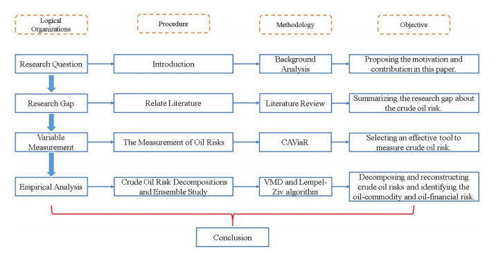
Crude oil markets have become increasingly uncertain. To study them, we first employ the decomposition-ensemble framework based on the variational mode decomposition (VMD) and Lempel–Ziv algorithms to assess the crude oil dual attributes. Three steps are involved: 1) conditional autoregressive value at risk measures the crude oil risk; 2) they are decomposed by the VMD algorithm into submodes; 3) the Lempel–Ziv algorithm is applied to analyze the crude oil risk for each, thereby identifying the oil commodity or oil financial risks. The results of the empirical analysis reveal significantly different amplitudes for the high- and low-frequency crude oil risk. By summarizing the crude oil risk components, we also conclude that the mean value for the oil commodity risk is 0.04, while that for the oil financial risk is 0. What is more, the oil commodity risk is highly related to downward trends in oil prices, while the oil financial risk exerts the same clustering effect as oil returns.
Citation: Hao Dong, Zhehao Huang. Decomposing and reconstructing dynamic risks in the crude oil market based on the VMD and Lempel–Ziv algorithms[J]. Electronic Research Archive, 2022, 30(12): 4674-4696. doi: 10.3934/era.2022237
Crude oil markets have become increasingly uncertain. To study them, we first employ the decomposition-ensemble framework based on the variational mode decomposition (VMD) and Lempel–Ziv algorithms to assess the crude oil dual attributes. Three steps are involved: 1) conditional autoregressive value at risk measures the crude oil risk; 2) they are decomposed by the VMD algorithm into submodes; 3) the Lempel–Ziv algorithm is applied to analyze the crude oil risk for each, thereby identifying the oil commodity or oil financial risks. The results of the empirical analysis reveal significantly different amplitudes for the high- and low-frequency crude oil risk. By summarizing the crude oil risk components, we also conclude that the mean value for the oil commodity risk is 0.04, while that for the oil financial risk is 0. What is more, the oil commodity risk is highly related to downward trends in oil prices, while the oil financial risk exerts the same clustering effect as oil returns.

| [1] |
R. Ahmed, S. M. Chaudhry, C. Kumpamool, C. Benjasak, Tail risk, systemic risk and spillover risk of crude oil and precious metals, Energy Econ., 112 (2022), 106063. https://doi.org/10.1016/j.eneco.2022.106063 doi: 10.1016/j.eneco.2022.106063

|
| [2] |
Z. Huang, H. Dong, S. Jia, Equilibrium pricing for carbon emission in response to the target of carbon emission peaking, Energy Econ., 112 (2022), 106160. https://doi.org/10.1016/j.eneco.2022.106160 doi: 10.1016/j.eneco.2022.106160
|
| [3] |
N. Nonejad, Forecasting crude oil price volatility out-of-sample using news-based geopolitical risk index: What forms of nonlinearity help improve forecast accuracy the most, Finance Res. Lett., 46 (2022), 102310. https://doi.org/10.1016/j.frl.2021.102310 doi: 10.1016/j.frl.2021.102310
|
| [4] |
Y. Zou, K. He, Forecasting crude oil risk using a multivariate multiscale convolutional neural network model, Mathematics, 10 (2022), 2413. https://doi.org/10.3390/math10142413 doi: 10.3390/math10142413
|
| [5] |
Q. Hu, T. Li, X. Li, H. Dong, Dynamic characteristics of oil attributes and their market effects, Energies, 14 (2021), 3927. https://doi.org/10.3390/en14133927. doi: 10.3390/en14133927
|
| [6] |
Y. Liu, Z. Li, Y. Yao, H. Dong, Asymmetry of risk evolution in crude oil market: From the perspective of dual attributes of oil, Energies, 14 (2021), 4063. https://doi.org/10.3390/en14134063 doi: 10.3390/en14134063
|
| [7] |
H. Min, X. Wang, Z. Li, Will oil price volatility cause market panic, Energies, 15 (2022), https://doi.org/10.3390/en15134629 doi: 10.3390/en15134629
|
| [8] |
W. Adekunle, A. M. Bagudo, M. Odumosu, S. B. Inuolaji, Predicting stock returns using crude oil prices: A firm level analysis of Nigeria's oil and gas sector, Resour. Policy, 68 (2020), 101708. https://doi.org/10.1016/j.resourpol.2020.101708 doi: 10.1016/j.resourpol.2020.101708
|
| [9] |
M. Asai, R. Gupta, M. McAleer, Forecasting volatility and co-volatility of crude oil and gold futures: Effects of leverage, jumps, spillovers, and geopolitical risks, Int. J. Forecast., 36 (2020), 933–948. https://doi.org/10.1016/j.ijforecast.2019.10.003 doi: 10.1016/j.ijforecast.2019.10.003
|
| [10] |
T. L. D. Huynh, T. Burggraf, M. A. Nasir, Financialisation of natural resources & instability caused by risk transfer in commodity markets, Resour. Policy, 66 (2020), 101620. https://doi.org/10.1016/j.resourpol.2020.101620 doi: 10.1016/j.resourpol.2020.101620
|
| [11] |
I. Chkir, K. Guesmi, A. B. Brayek, K. Naoui, Modelling the nonlinear relationship between oil prices, stock markets, and exchange rates in oil-exporting and oil-importing countries, Res. Int. Bus. Finance, 54 (2020), 101274. https://doi.org/10.1016/j.ribaf.2020.101274 doi: 10.1016/j.ribaf.2020.101274
|
| [12] |
T. Latunde, A. Lukman, D. D. Dare, Analysis of capital asset pricing model on deutsche bank energy commodity, Green Finance, 2 (2020), 20–34. https://doi.org/10.3934/GF.2020002 doi: 10.3934/GF.2020002
|
| [13] |
Z. Li, J. Zhong, Impact of economic policy uncertainty shocks on china's financial conditions, Finance Res. Lett., 35 (2020), 101303. https://doi.org/10.1016/j.frl.2019.101303 doi: 10.1016/j.frl.2019.101303
|
| [14] |
M. Ahmed, M. Azam, S. Bekiros, S. M. Hina, Are output fluctuations transitory or permanent? New evidence from a novel global multi-scale modeling approach, Quant. Finance Econ., 5 (2021), 373–396. https://doi.org/10.3934/QFE.2021017 doi: 10.3934/QFE.2021017
|
| [15] |
Z. Adams, S. Collot, M. Kartsakli, Have commodities become a financial asset? Evidence from ten years of Financialization, Energy Econ., 89 (2020), 104769. https://doi.org/10.1016/j.eneco.2020.104769 doi: 10.1016/j.eneco.2020.104769
|
| [16] |
R. L. D'Ecclesia, E. Magrini, P. Montalbano, U. Triulzi, Understanding recent oil price dynamics: A novel empirical approach, Energy Econ., 46 (2014), S11–S17. https://doi.org/10.1016/j.eneco.2014.10.005 doi: 10.1016/j.eneco.2014.10.005
|
| [17] |
K. Lang, B. R. Auer, The economic and financial properties of crude oil: A review, N. Am. J. Econ. Finance, 52 (2020), 100914. https://doi.org/10.1016/j.najef.2019.01.011 doi: 10.1016/j.najef.2019.01.011
|
| [18] |
K. S. Peng, G. F. Yan, A survey on deep learning for financial risk prediction, Quant. Finance Econ., 5 (2021), 716–737. https://doi.org/10.3934/QFE.2021032 doi: 10.3934/QFE.2021032
|
| [19] |
C. T. Albulescu, A. N. Ajmi, Oil price and US dollar exchange rate: Change detection of bi-directional causal impact, Energy Econ., 100 (2021), 105385. https://doi.org/10.1016/j.eneco.2021.105385 doi: 10.1016/j.eneco.2021.105385
|
| [20] |
S. Huang, H. An, B. Lucey, How do dynamic responses of exchange rates to oil price shocks co-move? From a time-varying perspective, Energy Econ., 86 (2020), 104641. https://doi.org/10.1016/j.eneco.2019.104641 doi: 10.1016/j.eneco.2019.104641
|
| [21] |
W. Mensi, S. Hammoudeh, S. J. H. Shahzad, K. H. Al-Yahyaee, M. Shahbaz, Oil and foreign exchange market tail dependence and risk spillovers for MENA, emerging and developed countries: VMD decomposition based copulas, Energy Econ., 67 (2017), 476–495. https://doi.org/10.1016/j.eneco.2017.08.036 doi: 10.1016/j.eneco.2017.08.036
|
| [22] |
T. M. Awan, M. S. Khan, I. U. Hap, S. Kazmi, Oil and stock markets volatility during pandemic times: a review of G7 countries, Green Finance, 3 (2021), 15–27. https://doi.org/10.3934/GF.2021002 doi: 10.3934/GF.2021002
|
| [23] |
Z. Li, Z. Huang, H. Dong, The influential factors on outward foreign direct investment: evidence from the "The Belt and Road", Emerg. Mark. Finance Trade, 55 (2019), 3211–3226. https://doi.org/10.1080/1540496X.2019.1569512 doi: 10.1080/1540496X.2019.1569512
|
| [24] |
T. Li, X. Li, G. Liao, Business cycles and energy intensity. Evidence from emerging economies, Borsa Istanbul Rev., 22 (2022), 560–570. https://doi.org/10.1016/j.bir.2021.07.005 doi: 10.1016/j.bir.2021.07.005
|
| [25] |
G. Liao, Z. Li, Z. Du, Y. Liu, The heterogeneous interconnections between supply or demand side and oil risks, Energies, 12 (2019), 2226. https://doi.org/10.3390/en12112226 doi: 10.3390/en12112226
|
| [26] |
L. Kilian, Not all oil price shocks are alike: Disentangling demand and supply shocks in the crude oil market, Am. Econ. Rev., 99 (2009), 1053–1069. https://doi.org/10.1257/aer.99.3.1053 doi: 10.1257/aer.99.3.1053
|
| [27] |
P. Ballco, A. Gracia, Do market prices correspond with consumer demands? Combining market valuation and consumer utility for extra virgin olive oil quality attributes in a traditional producing country, J. Retailing Consum. Serv., 53 (2020), 101999. https://doi.org/10.1016/j.jretconser.2019.101999 doi: 10.1016/j.jretconser.2019.101999
|
| [28] |
H. Bloch, S. Rafiq, R. Salim, Economic growth with coal, oil and renewable energy consumption in China: Prospects for fuel substitution, Econ. Model., 44 (2015), 104–115. https://doi.org/10.1016/j.econmod.2014.09.017 doi: 10.1016/j.econmod.2014.09.017
|
| [29] |
C. Belu Mănescu, G. Nuño, Quantitative effects of the shale oil revolution, Energy Policy, 86 (2015), 855–866. https://doi.org/10.1016/j.enpol.2015.05.015 doi: 10.1016/j.enpol.2015.05.015
|
| [30] |
L. Chen, Z. Zhang, F. Chen, N. Zhou, A study on the relationship between economic growth and energy consumption under the new normal, Natl. Account. Rev., 1 (2019), 28–41. https://doi.org/10.3934/NAR.2019.1.28 doi: 10.3934/NAR.2019.1.28
|
| [31] |
A. Loutia, C. Mellios, K. Andriosopoulos, Do OPEC announcements influence oil prices, Energy Policy, 90 (2016), 262–272. https://doi.org/10.1016/j.enpol.2015.11.025 doi: 10.1016/j.enpol.2015.11.025
|
| [32] |
Y. Liu, H. Dong, P. Failler, The oil market reactions to OPEC's announcements, Energies, 12 (2019), 3238. https://doi.org/10.3390/en12173238 doi: 10.3390/en12173238
|
| [33] |
X. Ma, Y. Jin, Q. Dong, A generalized dynamic fuzzy neural network based on singular spectrum analysis optimized by brain storm optimization for short-term wind speed forecasting, Appl. Soft Comput., 54 (2017). https://doi.org/10.1016/j.asoc.2017.01.033 doi: 10.1016/j.asoc.2017.01.033
|
| [34] |
L. T. Zhao, Y. Wang, S. Q. Guo, G. R. Zeng, A novel method based on numerical fitting for oil price trend forecasting, Appl. Energy, 220 (2018), 154–163. https://doi.org/10.1016/j.apenergy.2018.03.060 doi: 10.1016/j.apenergy.2018.03.060
|
| [35] |
Y. Huang, X. Dai, Q. Wang, D. Zhou, A hybrid model for carbon price forecasting using GARCH and long short-term memory network, Appl. Energy, 285 (2021), 116485. https://doi.org/10.1016/j.apenergy.2021.116485 doi: 10.1016/j.apenergy.2021.116485
|
| [36] |
L. Tang, S. Wang, K. He, S. Wang, A novel mode-characteristic-based decomposition ensemble model for nuclear energy consumption forecasting, Ann. Oper. Res., 234 (2015), 111–132. https://doi.org/10.1007/s10479-014-1595-5 doi: 10.1007/s10479-014-1595-5
|
| [37] |
S. Chen, S. Liu, R. Cai, Y. Zhang, The factors that influence exchange-rate risk: Evidence in China, Emerg. Mark. Finance Trade, 56 (2020), 1275–1292. https://doi.org/10.1080/1540496X.2019.1636229 doi: 10.1080/1540496X.2019.1636229
|
| [38] |
Z. Li, H. Dong, C. Floros, A. Charemis, P. Failler, Re-examining Bitcoin Volatility: A CAViaR-based Approach, Emerg. Mark. Finance Trade, 58 (2022), 1320–1338. https://doi.org/10.1080/1540496X.2021.1873127 doi: 10.1080/1540496X.2021.1873127
|
| [39] |
Z. Li, Z. Huang, P. Failler, Dynamic correlation between crude oil price and investor sentiment in China: Heterogeneous and asymmetric effect, Energies, 15 (2022), 687. https://doi.org/10.3390/en15030687 doi: 10.3390/en15030687
|
| [40] |
B. Wu, L. Wang, S. X. Lv, Y. R. Zeng, Effective crude oil price forecasting using new text-based and big-data-driven model, Measurement, 168 (2021), 108468. https://doi.org/10.1016/j.measurement.2020.108468 doi: 10.1016/j.measurement.2020.108468
|
| [41] |
M. Carreras-Simó, G. Coenders, The relationship between asset and capital structure: a compositional approach with panel vector autoregressive models, Quant. Finance Econ., 5 (2021), 571–590. https://doi.org/10.3934/QFE.2021025 doi: 10.3934/QFE.2021025
|
| [42] |
H. B. Ghassan, H. R. AlHajhoj, Long run dynamic volatilities between OPEC and non-OPEC crude oil prices, Appl. Energy, 169 (2016), 384–394. https://doi.org/10.1016/j.apenergy.2016.02.057 doi: 10.1016/j.apenergy.2016.02.057
|
| [43] |
C. Baumeister, L. Kilian, Forecasting the real price of oil in a changing world: A forecast combination approach, J. Bus. Econ. Stat., 33 (2015), 338–351. https://doi.org/10.1080/07350015.2014.949342 doi: 10.1080/07350015.2014.949342
|
| [44] |
Y. L. Wu, S. Y. Ma, Impact of COVID-19 on energy prices and main macroeconomic indicators—evidence from China's energy market, Green Finance, 3 (2021), 383–402. https://doi.org/10.3934/GF.2021019 doi: 10.3934/GF.2021019
|
| [45] |
R. F. Engle, S. Manganelli, CAViaR: Conditional autoregressive value at risk by regression quantiles, J. Bus. Econ. Stat., 22 (2004), 367–381. https://doi.org/10.1198/073500104000000370 doi: 10.1198/073500104000000370
|
| [46] |
K. Dragomiretskiy, D. Zosso, Variational mode decomposition, IEEE Trans. Signal Process., 62 (2014), 531–544. https://doi.org/10.1109/TSP.2013.2288675 doi: 10.1109/TSP.2013.2288675
|
| [47] |
T. Atalla, F. Joutz, A. Pierru, Does disagreement among oil price forecasters reflect volatility? Evidence from the ECB surveys, Int. J. Forecast., 32 (2016), 1178–1192. https://doi.org/10.1016/j.ijforecast.2015.09.009 doi: 10.1016/j.ijforecast.2015.09.009
|
| [48] |
J. L. Zhang, Y. J. Zhang, L. Zhang, A novel hybrid method for crude oil price forecasting, Energy Econ., 49 (2015), 649–659. https://doi.org/10.1016/j.eneco.2015.02.018 doi: 10.1016/j.eneco.2015.02.018
|
| [49] |
K. He, G. K. F. Tso, Y. Zou, J. Liu, Crude oil risk forecasting: New evidence from multiscale analysis approach, Energy Econ., 76 (2018), 574–583. https://doi.org/10.1016/j.eneco.2018.10.001 doi: 10.1016/j.eneco.2018.10.001
|
| [50] |
M. Bernardi, L. Catania, Comparison of value-at-risk models using the MCS approach, Comput. Stat., 31 (2016), 579–608. https://doi.org/10.1007/s00180-016-0646-6. doi: 10.1007/s00180-016-0646-6
|
| [51] |
F. M. Longin, The asymptotic distribution of extreme stock market returns, J. Bus., 69 (1996), 383–408. https://doi.org/10.1086/209695 doi: 10.1086/209695
|
| [52] |
J. D. Cabedo, I. Moya, Estimating oil price "Value at Risk" using the historical simulation approach, Energy Econ., 25 (2003), 239–253. https://doi.org/10.1016/S0140-9883(02)00111-1 doi: 10.1016/S0140-9883(02)00111-1
|
| [53] |
F. Ferraty, A. Quintela-Del-Río, Conditional VAR and expected shortfall: A new functional approach, Econom. Rev., 35 (2016), 263–292. https://doi.org/10.1080/07474938.2013.807107 doi: 10.1080/07474938.2013.807107
|
| [54] |
K. Gkillas, P. Katsiampa, An application of extreme value theory to cryptocurrencies, Econ. Lett., 164 (2018), 109–111. https://doi.org/10.1016/j.econlet.2018.01.020 doi: 10.1016/j.econlet.2018.01.020
|
| [55] |
Z. Li, H. Dong, Z. Huang, P. Failler, Asymmetric effects on risks of virtual financial assets (VFAs) in different regimes: A case of bitcoin. Quant. Finance Econ., 2 (2018), 860–883. https://doi.org/10.3934/QFE.2018.4.860 doi: 10.3934/QFE.2018.4.860
|
| [56] |
A. Tsoukala, G. Tsiotas, Assessing green bond risk: an empirical investigation, Green Finance, 3 (2021), 222–252. https://doi.org/10.3934/GF.2021012 doi: 10.3934/GF.2021012
|
| [57] |
L. T. Zhao, K. Liu, X. L. Duan, M. F. Li, Oil price risk evaluation using a novel hybrid model based on time-varying long memory, Energy Econ., 81 (2019), 70–78. https://doi.org/10.1016/j.eneco.2019.03.019 doi: 10.1016/j.eneco.2019.03.019
|
| [58] |
L. Yang, S. Hamori, Forecasts of value-at-risk and expected shortfall in the crude oil market: A wavelet-based semiparametric approach, Energies, 13 (2020), 3700. https://doi.org/10.3390/en13143700. doi: 10.3390/en13143700
|
| [59] |
D. Valenti, M. Manera, A. Sbuelz, Interpreting the oil risk premium: Do oil price shocks matter, Energy Econ., 91 (2020), 104906. https://doi.org/10.1016/j.eneco.2020.104906 doi: 10.1016/j.eneco.2020.104906
|
| [60] |
A. Drakos, G. P. Kouretas, L. Zarangas, Predicting conditional autoregressive Value-at-Risk for stock markets during tranquil and turbulent periods, J. Financ. Risk Manage., 4 (2015), 168. https://doi.org/10.4236/jfrm.2015.43014 doi: 10.4236/jfrm.2015.43014
|
| [61] |
J. Jeon, J. W. Taylor, Using CAViaR models with implied volatility for value-at-risk estimation, J. Forecast., 32 (2013), 62–74. https://doi.org/10.1002/for.1251 doi: 10.1002/for.1251
|
| [62] |
Z. Li, Y. Wang, Z. Huang, Risk connectedness heterogeneity in the cryptocurrency markets, Front. Phys., 8 (2020), 104906. https://doi.org/10.3389/fphy.2020.00243 doi: 10.3389/fphy.2020.00243
|
| [63] |
X. Meng, J. W. Taylor, An approximate long-memory range-based approach for value at risk estimation, Int. J. Forecast., 34 (2018), 377–388. https://doi.org/10.1016/j.ijforecast.2017.11.007 doi: 10.1016/j.ijforecast.2017.11.007
|
| [64] | M. Youssef, L. Belkacem, K. Mokni, Value-at-Risk estimation of energy commodities: A long-memory GARCH-EVT approach, Energy Econ., 51 (2015), 99–110. https://doi.org/0.1016/j.eneco.2015.06.010 |
| [65] |
H. Dong, Y. Liu, J. Chang, The heterogeneous linkage of economic policy uncertainty and oil return risks, Green Finance, 1 (2019), 46–66. https://doi.org/10.3934/GF.2019.1.46 doi: 10.3934/GF.2019.1.46
|
| [66] |
D. Wen, L. Liu, C. Ma, Y. Wang, Extreme risk spillovers between crude oil prices and the US exchange rate: Evidence from oil-exporting and oil-importing countries, Energy, 212 (2020), 118740. https://doi.org/10.1016/j.energy.2020.118740 doi: 10.1016/j.energy.2020.118740
|
| [67] |
B. Zhu, A novel multiscale ensemble carbon price prediction model integrating empirical mode decomposition, genetic algorithm and artificial neural network, Energies, 5 (2012), 355–370. https://doi.org/10.3390/en5020355 doi: 10.3390/en5020355
|
| [68] |
B. Zhu, D. Han, P. Wang, Z. Wu, T. Zhang, Y. M. Wei, Forecasting carbon price using empirical mode decomposition and evolutionary least squares support vector regression, Appl. Energy, 191 (2017), 521–530. https://doi.org/10.1016/j.apenergy.2017.01.076 doi: 10.1016/j.apenergy.2017.01.076
|
| [69] |
W. Li, C. Lu, The research on setting a unified interval of carbon price benchmark in the national carbon trading market of China, Appl. Energy, 155 (2015), 728–739. https://doi.org/10.1016/j.apenergy.2015.06.018 doi: 10.1016/j.apenergy.2015.06.018
|
| [70] |
B. Zhu, S. Ye, K. He, J. Chevallier, R. Xie, Measuring the risk of European carbon market: an empirical mode decomposition-based value at risk approach, Ann. Oper. Res., 281 (2019), 373–395. https://doi.org/10.1007/s10479-018-2982-0 doi: 10.1007/s10479-018-2982-0
|
| [71] |
G. Sun, T. Chen, Z. Wei, Y. Sun, H. Zang, S. Chen, A carbon price forecasting model based on variational mode decomposition and spiking neural networks, Energies, 9 (2016), 54. https://doi.org/10.3390/en9010054 doi: 10.3390/en9010054
|
| [72] |
Y. Zou, L. Yu, G. K. F. Tso, K. He, Risk forecasting in the crude oil market: A multiscale convolutional neural network approach, Physica A, 541 (2020), 123360. https://doi.org/10.1016/j.physa.2019.123360 doi: 10.1016/j.physa.2019.123360
|
| [73] |
Y. Hao, C. Tian, A hybrid framework for carbon trading price forecasting: The role of multiple influence factor, J. Clean Prod., 262 (2020), 120378. https://doi.org/10.1016/j.jclepro.2020.120378 doi: 10.1016/j.jclepro.2020.120378
|
| [74] |
H. Lu, X. Ma, K. Huang, M. Azimi, Carbon trading volume and price forecasting in China using multiple machine learning models, J. Clean Prod., 249 (2020), 119386. https://doi.org/10.1016/j.jclepro.2019.119386 doi: 10.1016/j.jclepro.2019.119386
|
| [75] |
C. P. Cristescu, C. Stan, E. I. Scarlat, The dynamics of exchange rate time series and the chaos game, Physica A, 388 (2009), 4845–4855. https://doi.org/10.1016/j.physa.2009.08.005 doi: 10.1016/j.physa.2009.08.005
|
| [76] |
R. Li, Y. Hu, J. Heng, X. Chen, A novel multiscale forecasting model for crude oil price time series, Technol. Forecasting Social Change, 173 (2021), 121181. https://doi.org/10.1016/j.techfore.2021.121181 doi: 10.1016/j.techfore.2021.121181
|
| [77] |
X. Yan, D. She, Y. Xu, M. Jia, Application of generalized composite multiscale Lempel-Ziv complexity in identifying wind turbine gearbox faults, Entropy, 23 (2021), 1372w. https://doi.org/10.3390/e23111372 doi: 10.3390/e23111372
|
| [78] |
J. B. Gao, Y. F. Hou, F. L. Fan, F. Y. Liu, Complexity changes in the US and China's stock markets: Differences, causes, and wider social implications, Entropy, 22 (2020), 75. https://doi.org/10.3390/e22010075 doi: 10.3390/e22010075
|
| [79] |
A. Lempel, J. Ziv, On the complexity of finite Sequences, IEEE Trans. Inf. Theory, 22 (1976), 75–81. https://doi.org/10.1109/TIT.1976.1055501 doi: 10.1109/TIT.1976.1055501
|
| [80] |
S. Chen, J. Zhong, P. Failler, Does China transmit financial cycle spillover effects to the G7 countries, Econ. Res. Ekon Istraz., 35 (2021), 5184–5201. https://doi.org/10.1080/1331677X.2021.2025123 doi: 10.1080/1331677X.2021.2025123
|
| [81] |
Z. Li, H. Chen, B. Mo, Can digital finance promote urban innovation? Evidence from China, Borsa Istanb. Rev., (2022), forthcoming. https://doi.org/10.1016/j.bir.2022.10.006 doi: 10.1016/j.bir.2022.10.006
|


Figures(10) / Tables(1)
Hao Dong, Zhehao Huang. Decomposing and reconstructing dynamic risks in the crude oil market based on the VMD and Lempel–Ziv algorithms[J]. Electronic Research Archive, 2022, 30(12): 4674-4696. doi: 10.3934/era.2022237


 DownLoad: