Symmetry analysis of an acid-mediated cancer invasion model

Juya Cui; Ben Gao; Juya Cui; Ben Gao

doi:10.3934/math.2022930

AIMS Mathematics

2022, Volume 7, Issue 9: 16949-16961. doi: 10.3934/math.2022930

Previous Article Next Article

Research article

Symmetry analysis of an acid-mediated cancer invasion model

Juya Cui ^{1
,
,},
Ben Gao ²

1.
Department of Lymphoma, Shanxi Bethune Hospital, Shanxi Academy of Medical Sciences, Taiyuan, Shanxi 030032, China
2.
College of Mathematics, Taiyuan University of Technology, Taiyuan, Shanxi 030024, China

Received: 21 February 2022 Revised: 30 June 2022 Accepted: 11 July 2022 Published: 18 July 2022
MSC : 35E05, 35J05, 43A80

Under investigation in this paper is a reaction-diffusion system, which describes acid-mediated tumor growth. First, in view of Lie group analysis, infinitesimal generators of the considered system are presented. At the same time, some group invariant solutions are computed using reduced equations. In particular, we construct explicit solutions by applying the power-series method. Furthermore, the convergence of the solutions of the power-series is certificated. Finally, the stability behavior of the model can be understood by analyzing the solutions of different parameters.
- tumor growth,
- symmetries,
- power-series solutions
Citation: Juya Cui, Ben Gao. Symmetry analysis of an acid-mediated cancer invasion model[J]. AIMS Mathematics, 2022, 7(9): 16949-16961. doi: 10.3934/math.2022930

Related Papers:

Abstract

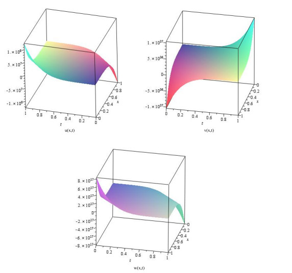
Under investigation in this paper is a reaction-diffusion system, which describes acid-mediated tumor growth. First, in view of Lie group analysis, infinitesimal generators of the considered system are presented. At the same time, some group invariant solutions are computed using reduced equations. In particular, we construct explicit solutions by applying the power-series method. Furthermore, the convergence of the solutions of the power-series is certificated. Finally, the stability behavior of the model can be understood by analyzing the solutions of different parameters.

References

[1]	D. S. Jones, B. D. Sleeman, Differential equations and mathematical biology, Chapman and Hall/CRC, 2003.
[2]	P. Veeresha, E. Ilhan, D. G. Prakasha, H. M. Baskonus, W. Gao, Regarding on the fractional mathematical model of tumour invasion and metastasis, CMES-Comp. Model. Eng., 127 (2021), 1013–1036. https://doi.org/10.32604/cmes.2021.014988 doi: 10.32604/cmes.2021.014988
[3]	A. Bertuzzi, A. Fasano, A. Gandolfi, C. Sinisgalli, ATP production and necrosis formation in a tumour spheroid model, Math. Model. Nat. Phenom., 2 (2007), 30–46. https://doi.org/10.1051/mmnp:2007002 doi: 10.1051/mmnp:2007002
[4]	R. Venkatasubramanian, M. A. Henson, N. S. Forbes, Incorporating energy metabolism into a growth model of multicellular tumor spheroids, J. Theor. Biol., 242 (2006), 440–453. https://doi.org/10.1016/j.jtbi.2006.03.011 doi: 10.1016/j.jtbi.2006.03.011
[5]	T. Telksnys, I. Timofejeva, Z. Navickas, R. Marcinkevicius, R. Mickevicius, M. Ragulskis, Solitary solutions to an androgen-deprivation prostate cancer treatment model, Math. Method. Appl. Sci., 43 (2020), 3995–4006. https://doi.org/10.1002/mma.6168 doi: 10.1002/mma.6168
[6]	N. Bellomo, N. K. Li, P. K. Maini, On the foundations of cancer modelling: selected topics, speculations, and perspectives, Math. Mod. Meth. Appl. S., 18 (2008), 593–646. https://doi.org/10.1142/S0218202508002796 doi: 10.1142/S0218202508002796
[7]	T. Telksnys, Z. Navickas, M. A. F. Sanjuan, R. Marcinkevicius, M. Ragulskis, Kink solitary solutions to a hepatitis C evolution model, Discrete Cont. Dyn. Syst. B, 25 (2020), 4427–4447. https://doi.org/10.3934/dcdsb.2020106 doi: 10.3934/dcdsb.2020106
[8]	T. Telksnys, Z. Navickas, R. Marcinkevicius, M. S. Cao, M. Ragulskis, Homoclinic and heteroclinic solutions to a hepatitis C evolution model, Open Math., 16 (2018), 1537–1555. https://doi.org/10.1515/math-2018-0130 doi: 10.1515/math-2018-0130
[9]	R. A. Gatenby, E. T. Gawlinski, A reaction-diffusion model for cancer invasion, Cancer Res., 56 (1996), 5745–5753.
[10]	R. A. Gatenby, E. T. Gawlinski, The glycolytic phenotype in carcinogenesis and tumour invasion: insights through mathematical modelling, Cancer Res., 63 (2003), 3847–3854.
[11]	A. Fasano, M. A. Herrero, M. R. Rodrigo, Slow and fast invasion waves in a model of acid-mediated tumour growth, Math. Biosci., 220 (2009), 45–56. https://doi.org/10.1016/j.mbs.2009.04.001 doi: 10.1016/j.mbs.2009.04.001
[12]	B. Gao, Y. Zhang, Symmetry analysis of the time fractional Gaudrey-Dodd-Gibbon equation, Physica A, 525 (2019), 1058–1062. https://doi.org/10.1016/j.physa.2019.04.023 doi: 10.1016/j.physa.2019.04.023
[13]	Z. G. Wang, Symmetries and solutions of hyperbolic mean curvature flow with a constant forcing term, Appl. Math. Comput., 235 (2014), 560–566. https://doi.org/10.1016/j.amc.2013.12.134 doi: 10.1016/j.amc.2013.12.134
[14]	B. Gao, C. F. He, Analysis of a coupled short pulse system via symmetry method, Nonlinear Dyn., 90 (2017), 2627–2636. https://doi.org/10.1007/s11071-017-3827-0 doi: 10.1007/s11071-017-3827-0
[15]	J. H. Wang, Symmetries and solutions to geometrical flows, Sci. China Math., 56 (2013), 1689–1704. https://doi.org/10.1007/s11425-013-4635-8 doi: 10.1007/s11425-013-4635-8
[16]	P. J. Olver, Applications of Lie groups to differential equations, New York: Springer, 1993. https://doi.org/10.1007/978-1-4612-4350-2
[17]	G. W. Bluman, S. Kumei, Symmetries and differential equations, New York, NY: Springer, 1989. https://doi.org/10.1007/978-1-4757-4307-4
[18]	B. Gao, Y. X. Wang, Invariant solutions and nonlinear self-adjointness of the two-component Chaplygin gas equation, Discrete. Dyn. Nat. Soc., 2019 (2019), 9609357. https://doi.org/10.1155/2019/9609357 doi: 10.1155/2019/9609357
[19]	G. W. Bluman, S. C. Anco, Symmetry and integration methods for differential equations, New York, NY: Springer, 2002. https://doi.org/10.1007/b97380
[20]	N. H. Asmar, Partial differential equations with Fourier series and boundary value problems, Beijing: China Machine Press, 2005.
[21]	W. Rudin, Principles of mathematical analysis, Beijing: China Machine Press, 2004.

Reader Comments

Your name:*

Email:*
© 2022 the Author(s), licensee AIMS Press. This is an open access article distributed under the terms of the Creative Commons Attribution License (http://creativecommons.org/licenses/by/4.0)