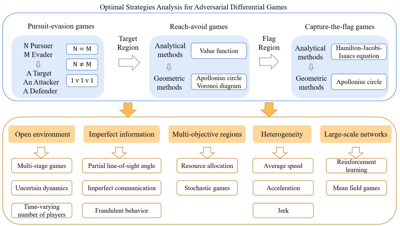
Optimal decision-making and winning-regions analysis in adversarial differential games are challenging theoretical problems because of the complex interactions between players. To solve these problems, we present an organized review for pursuit-evasion games, reach-avoid games and capture-the-flag games; we also outline recent developments in three types of games. First, we summarize recent results for pursuit-evasion games and classify them according to different numbers of players. As a special kind of pursuit-evasion games, target-attacker-defender games with an active target are analyzed from the perspectives of different speed ratios for players. Second, the related works for reach-avoid games and capture-the-flag games are compared in terms of analytical methods and geometric methods, respectively. These methods have different effects on the barriers and optimal strategy analysis between players. Future directions for the pursuit-evasion games, reach-avoid games, capture-the-flag games and their applications are discussed in the end.
Citation: Jiali Wang, Xin Jin, Yang Tang. Optimal strategy analysis for adversarial differential games[J]. Electronic Research Archive, 2022, 30(10): 3692-3710. doi: 10.3934/era.2022189
Optimal decision-making and winning-regions analysis in adversarial differential games are challenging theoretical problems because of the complex interactions between players. To solve these problems, we present an organized review for pursuit-evasion games, reach-avoid games and capture-the-flag games; we also outline recent developments in three types of games. First, we summarize recent results for pursuit-evasion games and classify them according to different numbers of players. As a special kind of pursuit-evasion games, target-attacker-defender games with an active target are analyzed from the perspectives of different speed ratios for players. Second, the related works for reach-avoid games and capture-the-flag games are compared in terms of analytical methods and geometric methods, respectively. These methods have different effects on the barriers and optimal strategy analysis between players. Future directions for the pursuit-evasion games, reach-avoid games, capture-the-flag games and their applications are discussed in the end.

| [1] |
R. Yan, Z. Shi, Y. Zhong, Task assignment for multiplayer reach–avoid games in convex domains via analytical barriers, IEEE Trans. Rob., 36 (2019), 107–124. https://doi.org/10.1109/TRO.2019.2935345 doi: 10.1109/TRO.2019.2935345

|
| [2] | E. Garcia, I. Weintraub, D. W. Casbeer, M. Pachter, Optimal strategies for the game of protecting a plane in 3-d, preprint, arXiv: 2202.01826. |
| [3] |
E. Garcia, D. W. Casbeer, M. Pachter, Optimal strategies of the differential game in a circular region, IEEE Control Syst. Lett., 4 (2019), 492–497. https://doi.org/10.1109/LCSYS.2019.2963173 doi: 10.1109/LCSYS.2019.2963173
|
| [4] |
J. Chen, W. Zha, Z. Peng, D. Gu, Multi-player pursuit–evasion games with one superior evader, Automatica, 71 (2016), 24–32. https://doi.org/10.1016/j.automatica.2016.04.012 doi: 10.1016/j.automatica.2016.04.012
|
| [5] |
K. Chen, W. He, Q. L. Han, M. Xue, Y. Tang, Leader selection in networks under switching topologies with antagonistic interactions, Automatica, 142 (2022), 110334. https://doi.org/10.1016/j.automatica.2022.110334 doi: 10.1016/j.automatica.2022.110334
|
| [6] |
Z. Li, X. Yu, J. Qiu, H. Gao, Cell division genetic algorithm for component allocation optimization in multifunctional placers, IEEE Trans. Ind. Inf., 18 (2021), 559–570. https://doi.org/10.1109/TⅡ.2021.3069459 doi: 10.1109/TⅡ.2021.3069459
|
| [7] |
Y. Tang, C. Zhao, J. Wang, C. Zhang, Q. Sun, W. Zheng, et al., An overview of perception and decision-making in autonomous systems in the era of learning, IEEE Trans. Neural Networks Learn. Syst., 2022. https://doi.org/10.1109/TNNLS.2022.3167688 doi: 10.1109/TNNLS.2022.3167688
|
| [8] |
E. Garcia, D. W. Casbeer, A. V. Moll, M. Pachter, Multiple pursuer multiple evader differential games, IEEE Trans. Autom. Control, 66 (2020), 2345–2350. https://doi.org/10.1109/TAC.2020.3003840 doi: 10.1109/TAC.2020.3003840
|
| [9] |
E. Garcia, D. W. Casbeer, M. Pachter, Optimal strategies for a class of multi-player reach-avoid differential games in 3d space, IEEE Rob. Autom. Lett., 5 (2020), 4257–4264, https://doi.org/10.1109/LRA.2020.2994023 doi: 10.1109/LRA.2020.2994023
|
| [10] |
H. Huang, J. Ding, W. Zhang, C. J. Tomlin, Automation-assisted capture-the-flag: A differential game approach, IEEE Trans. Control Syst. Technol., 23 (2014), 1014–1028. https://doi.org/10.1109/TCST.2014.2360502 doi: 10.1109/TCST.2014.2360502
|
| [11] | Z. Zhou, J. Huang, J. Xu, Y. Tang, Two-phase jointly optimal strategies and winning regions of the capture-the-flag game, in IECON 2021 – 47th Annual Conference of the IEEE Industrial Electronics Society, (2021), 1–6. https://doi.org/10.1109/IECON48115.2021.9589624 |
| [12] | E. Garcia, A. V. Moll, D. W. Casbeer, M. Pachter, Strategies for defending a coastline against multiple attackers, in 2019 IEEE 58th Conference on Decision and Control (CDC), (2019), 7319–7324. https://doi.org/10.1109/CDC40024.2019.9029340 |
| [13] | I. E. Weintraub, M. Pachter, E. Garcia, An introduction to pursuit-evasion differential games, in 2020 American Control Conference (ACC), (2020), 1049–1066. https://doi.org/10.23919/ACC45564.2020.9147205 |
| [14] |
T. Başar, A tutorial on dynamic and differential games, Dyn. Games Appl. Econ., (1986), 1–25. https://doi.org/10.1007/978-3-642-61636-5_1 doi: 10.1007/978-3-642-61636-5_1
|
| [15] |
S. S. Kumkov, S. L. Ménec, V. S. Patsko, Zero-sum pursuit-evasion differential games with many objects: survey of publications, Dyn. Games Appl., 7 (2017), 609–633. https://doi.org/10.1007/s13235-016-0209-z doi: 10.1007/s13235-016-0209-z
|
| [16] | R. Yan, Z. Shi, Y. Zhong, Defense game in a circular region, in 2017 IEEE 56th Annual Conference on Decision and Control (CDC), (2017), 5590–5595. https://doi.org/10.1109/CDC.2017.8264502 |
| [17] | I. E. Weintraub, A. V. Moll, E. Garcia, D. Casbeer, Z. J. Demers, M. Pachter, Maximum observation of a faster non-maneuvering target by a slower observer, in 2020 American Control Conference (ACC), (2020), 100–105. https://doi.org/10.23919/ACC45564.2020.9147340 |
| [18] |
J. Wang, Y. Hong, J. Wang, J. Xu, Y. Tang, Q. L. Han, et al., Cooperative and competitive multi-agent systems:from optimization to games, IEEE/CAA J. Autom. Sin., 9 (2022), 763–783. https://doi.org/10.1109/JAS.2022.105506 doi: 10.1109/JAS.2022.105506
|
| [19] | A. A. Al-Talabi, Multi-player pursuit-evasion differential game with equal speed, in 2017 International Automatic Control Conference (CACS), (2017), 1–6. https://doi.org/10.1109/CACS.2017.8284276 |
| [20] |
D. Shishika, J. Paulos, V. Kumar, Cooperative team strategies for multi-player perimeter-defense games, IEEE Rob. Autom. Lett., 5 (2020), 2738–2745. https://doi.org/10.1109/LRA.2020.2972818 doi: 10.1109/LRA.2020.2972818
|
| [21] |
E. Garcia, Z. E. Fuchs, D. Milutinovic, D. W. Casbeer, M. Pachter, A geometric approach for the cooperative two-pursuer one-evader differential game, IFAC-PapersOnLine, 50 (2017), 15209–15214. https://doi.org/10.1016/j.ifacol.2017.08.2366 doi: 10.1016/j.ifacol.2017.08.2366
|
| [22] |
A. V. Moll, D. Casbeer, E. Garcia, D. Milutinović, M. Pachter, The multi-pursuer single-evader game, J. Intell. Rob. Syst., 96 (2019), 193–207. https://doi.org/10.1007/s10846-018-0963-9 doi: 10.1007/s10846-018-0963-9
|
| [23] | E. Garcia, S. D. Bopardikar, Cooperative containment of a high-speed evader, in 2021 American Control Conference (ACC), (2021), 4698–4703. https://doi.org/10.23919/ACC50511.2021.9483097 |
| [24] | E. Garcia, D. W. Casbeer, D. Tran, M. Pachter, A differential game approach for beyond visual range tactics, in 2021 American Control Conference (ACC), (2021), 3210–3215. https://doi.org/10.23919/ACC50511.2021.9482650 |
| [25] |
Y. Xu, H. Yang, B. Jiang, M. M. Polycarpou, Multi-player pursuit-evasion differential games with malicious pursuers, IEEE Trans. Autom. Control, 2022. https://doi.org/10.1109/TAC.2022.3168430 doi: 10.1109/TAC.2022.3168430
|
| [26] |
W. Lin, Z. Qu, M. A. Simaan, Nash strategies for pursuit-evasion differential games involving limited observations, IEEE Trans. Aerosp. Electron. Syst., 51 (2015), 1347–1356. https://doi.org/10.1109/TAES.2014.130569 doi: 10.1109/TAES.2014.130569
|
| [27] | M. Pachter, E. Garcia, D. W. Casbeer, Active target defense differential game, in 2014 52nd Annual Allerton Conference on Communication, Control, and Computing (Allerton), (2014), 46–53. https://doi.org/10.1109/ALLERTON.2014.7028434 |
| [28] |
E. Garcia, D. W. Casbeer, M. Pachter, Active target defense using first order missile models, Automatica, 78 (2017), 139–143. https://doi.org/10.1016/j.automatica.2016.12.032 doi: 10.1016/j.automatica.2016.12.032
|
| [29] | M. Coon, D. Panagou, Control strategies for multiplayer target-attacker-defender differential games with double integrator dynamics, in 2017 IEEE 56th Annual Conference on Decision and Control (CDC), (2017), 1496–1502. https://doi.org/10.1109/CDC.2017.8263864 |
| [30] | I. E. Weintraub, E. Garcia, M. Pachter, A kinematic rejoin method for active defense of non-maneuverable aircraft, in 2018 Annual American Control Conference (ACC), (2018), 6533–6538. https://doi.org/10.23919/ACC.2018.8431129 |
| [31] |
E. Garcia, D. W. Casbeer, M. Pachter, Design and analysis of state-feedback optimal strategies for the differential game of active defense, IEEE Trans. Autom. Control, 64 (2018), 553–568. https://doi.org/10.1109/TAC.2018.2828088 doi: 10.1109/TAC.2018.2828088
|
| [32] | E. Garcia, D. W. Casbeer, M. Pachter, Optimal target capture strategies in the target-attacker-defender differential game, in 2018 Annual American Control Conference (ACC), (2018), 68–73. https://doi.org/10.23919/ACC.2018.8431715 |
| [33] |
E. Garcia, D. W. Casbeer, M. Pachter, The complete differential game of active target defense, J. Optim. Theory Appl., 191 (2021), 675–699. https://doi.org/10.1007/s10957-021-01816-z doi: 10.1007/s10957-021-01816-z
|
| [34] |
E. Garcia, D. W. Casbeer, M. Pachter, Pursuit in the presence of a defender, Dyn. Games Appl., 9 (2019), 652–670. https://doi.org/10.1007/s13235-018-0271-9 doi: 10.1007/s13235-018-0271-9
|
| [35] |
M. Pachter, E. Garcia, D. W. Casbeer, Toward a solution of the active target defense differential game, Dyn. Games Appl., 9 (2019), 165–216. https://doi.org/10.1007/s13235-018-0250-1 doi: 10.1007/s13235-018-0250-1
|
| [36] |
E. Garcia, Cooperative target protection from a superior attacker, Automatica, 131 (2021), 109696. https://doi.org/10.1016/j.automatica.2021.109696 doi: 10.1016/j.automatica.2021.109696
|
| [37] | M. Pachter, E. Garcia, R. Anderson, D. W. Casbeer, K. Pham, Maximizing the target's longevity in the active target defense differential game, in 2019 18th European Control Conference (ECC), (2019), 2036–2041. https://doi.org/10.23919/ECC.2019.8795650 |
| [38] | E. Garcia, D. W. Casbeer, M. Pachter, Defense of a target against intelligent adversaries: A linear quadratic formulation, in 2020 IEEE Conference on Control Technology and Applications (CCTA), (2020), 619–624. https://doi.org/10.1109/CCTA41146.2020.9206368 |
| [39] |
E. Garcia, D. W. Casbeer, M. Pachter, Cooperative strategies for optimal aircraft defense from an attacking missile, J. Guid., Control, Dyn., 38 (2015), 1510–1520. https://doi.org/10.2514/1.G001083 doi: 10.2514/1.G001083
|
| [40] |
L. Liang, F. Deng, Z. Peng, X. Li, W. Zha, A differential game for cooperative target defense, Automatica, 102 (2019), 58–71. https://doi.org/10.1016/j.automatica.2018.12.034 doi: 10.1016/j.automatica.2018.12.034
|
| [41] |
Z. Zhou, J. Ding, H. Huang, R. Takei, C. Tomlin, Efficient path planning algorithms in reach-avoid problems, Automatica, 89 (2018), 28–36. https://doi.org/10.1016/j.automatica.2017.11.035 doi: 10.1016/j.automatica.2017.11.035
|
| [42] | P. Shi, W. Sun, X. Yang, I. J. Rudas, H. Gao, Master-slave synchronous control of dual-drive gantry stage with cogging force compensation, IEEE Trans. Syst. Man Cybern.: Syst., https://doi.org/10.1109/TSMC.2022.3176952 |
| [43] | J. Lorenzetti, M. Chen, B. Landry, M. Pavone, Reach-avoid games via mixed-integer second-order cone programming, in 2018 IEEE Conference on Decision and Control (CDC), (2018), 4409–4416. https://doi.org/10.1109/CDC.2018.8619382 |
| [44] |
R. Isaacs, Differential games: Their scope, nature, and future, J. Optim. Theory Appl., 3 (1969), 283–295. https://doi.org/10.1007/BF00931368 doi: 10.1007/BF00931368
|
| [45] |
R. Yan, Z. Shi, Y. Zhong, Guarding a subspace in high-dimensional space with two defenders and one attacker, IEEE Trans. Cybern., 2020. https://doi.org/10.1109/TCYB.2020.3015031 doi: 10.1109/TCYB.2020.3015031
|
| [46] | R. Yan, Z. Shi, Y. Zhong, Construction of the barrier for reach-avoid differential games in three-dimensional space with four equal-speed players, in 2019 IEEE 58th Conference on Decision and Control (CDC), (2019), 4067–4072. https://doi.org/10.1109/CDC40024.2019.9029495 |
| [47] |
K. Margellos, J. Lygeros, Hamilton–jacobi formulation for reach–avoid differential games, IEEE Trans. Autom. Control, 56 (2011), 1849–1861. https://doi.org/10.1109/TAC.2011.2105730 doi: 10.1109/TAC.2011.2105730
|
| [48] | J. F. Fisac, M. Chen, C. J. Tomlin, S. S. Sastry, Reach-avoid problems with time-varying dynamics, targets and constraints, in HSCC '15: Proceedings of the 18th International Conference on Hybrid Systems: Computation and Control, (2015), 11–20. https://doi.org/10.1145/2728606.2728612 |
| [49] |
M. Chen, Z. Zhou, C. J. Tomlin, Multiplayer reach-avoid games via pairwise outcomes, IEEE Trans. Autom. Control, 62 (2016), 1451–1457. https://doi.org/10.1109/TAC.2016.2577619 doi: 10.1109/TAC.2016.2577619
|
| [50] | V. Mnih, K. Kavukcuoglu, D. Silver, A. Graves, I. Antonoglou, D. Wierstra, et al., Playing atari with deep reinforcement learning, preprint, arXiv: 1312.5602. |
| [51] | S. Bansal, C. J. Tomlin, Deepreach: A deep learning approach to high-dimensional reachability, in 2021 IEEE International Conference on Robotics and Automation (ICRA), (2021), 1817–1824. https://doi.org/10.1109/ICRA48506.2021.9561949 |
| [52] | J. Li, D. Lee, S. Sojoudi, C. J. Tomlin, Infinite-horizon reach-avoid zero-sum games via deep reinforcement learning, preprint, arXiv: 2203.10142. |
| [53] | K. C. Hsu, V. R. Royo, C. J. Tomlin, J. F. Fisac, Safety and liveness guarantees through reach-avoid reinforcement learning, preprint, arXiv: 2112.12288. |
| [54] | E. Garcia, D. W. Casbeer, A. V. Moll, M. Pachter, Cooperative two-pursuer one-evader blocking differential game, in 2019 American Control Conference (ACC), (2019), 2702–2709. https://doi.org/10.23919/ACC.2019.8814294 |
| [55] |
R. Yan, X. Duan, Z. Shi, Y. Zhong, F. Bullo, Matching-based capture strategies for 3d heterogeneous multiplayer reach-avoid differential games, Automatica, 140 (2022), 110207. https://doi.org/10.1016/j.automatica.2022.110207 doi: 10.1016/j.automatica.2022.110207
|
| [56] |
J. Selvakumar, E. Bakolas, Feedback strategies for a reach-avoid game with a single evader and multiple pursuers, IEEE Trans. Cybern., 51 (2019), 696–707. https://doi.org/10.1109/TCYB.2019.2914869 doi: 10.1109/TCYB.2019.2914869
|
| [57] | E. Garcia, D. W. Casbeer, M. Pachter, J. W. Curtis, E. Doucette, A two-team linear quadratic differential game of defending a target, in 2020 American Control Conference (ACC), (2020), 1665–1670. https://doi.org/10.23919/ACC45564.2020.9147665 |
| [58] |
S. D. Bopardikar, F. Bullo, J. P. Hespanha, A cooperative homicidal chauffeur game, Automatica, 45 (2009), 1771–1777. https://doi.org/10.1016/j.automatica.2009.03.014 doi: 10.1016/j.automatica.2009.03.014
|
| [59] |
R. Lopez-Padilla, R. Murrieta-Cid, I. Becerra, G. Laguna, S. M. LaValle, Optimal navigation for a differential drive disc robot: A game against the polygonal environment, J. Intell. Rob. Syst., 89 (2018), 211–250. https://doi.org/10.1007/s10846-016-0433-1 doi: 10.1007/s10846-016-0433-1
|
| [60] |
A. Pierson, Z. Wang, M. Schwager, Intercepting rogue robots: An algorithm for capturing multiple evaders with multiple pursuers, IEEE Rob. Autom. Lett., 2 (2016), 530–537. https://doi.org/10.1109/LRA.2016.2645516 doi: 10.1109/LRA.2016.2645516
|
| [61] |
Z. Zhou, W. Zhang, J. Ding, H. Huang, D. M. Stipanović, C. J. Tomlin, Cooperative pursuit with voronoi partitions, Automatica, 72 (2016), 64–72. https://doi.org/10.1016/j.automatica.2016.05.007 doi: 10.1016/j.automatica.2016.05.007
|
| [62] |
E. Bakolas, P. Tsiotras, Relay pursuit of a maneuvering target using dynamic voronoi diagrams, Automatica, 48 (2012), 2213–2220. https://doi.org/10.1016/j.automatica.2012.06.003 doi: 10.1016/j.automatica.2012.06.003
|
| [63] |
R. Yan, Z. Shi, Y. Zhong, Reach-avoid games with two defenders and one attacker: An analytical approach, IEEE Trans. Cybern., 49 (2018), 1035–1046. https://doi.org/10.1109/TCYB.2018.2794769 doi: 10.1109/TCYB.2018.2794769
|
| [64] |
R. Yan, Z. Shi, Y. Zhong, Cooperative strategies for two-evader-one-pursuer reach-avoid differential games, Int. J. Syst. Sci., 52 (2021), 1894–1912. https://doi.org/10.1080/00207721.2021.1872116 doi: 10.1080/00207721.2021.1872116
|
| [65] |
J. Wang, J. Huang, Y. Tang, Swarm intelligence capture-the-flag game with imperfect information based on deep reinforcement learning, Sci. Sin. Technol., 2021. https://doi.org/10.1360/SST-2021-0382 doi: 10.1360/SST-2021-0382
|
| [66] |
I. M. Mitchell, A. M. Bayen, C. J. Tomlin, A time-dependent hamilton-jacobi formulation of reachable sets for continuous dynamic games, IEEE Trans. Autom. Control, 50 (2005), 947–957. https://doi.org/10.1109/TAC.2005.851439 doi: 10.1109/TAC.2005.851439
|
| [67] | E. Garcia, D. W. Casbeer, M. Pachter, The capture-the-flag differential game, in 2018 IEEE Conference on Decision and Control (CDC), (2018), 4167–4172. https://doi.org/10.1109/CDC.2018.8619026 |
| [68] | M. Pachter, D. W. Casbeer, E. Garcia, Capture-the-flag: A differential game, in 2020 IEEE Conference on Control Technology and Applications (CCTA), (2020), 606–610. https://doi.org/10.1109/CCTA41146.2020.9206333 |
| [69] |
Z. Liu, W. Lin, X. Yu, J. J. Rodríguez-Andina, H. Gao, Approximation-free robust synchronization control for dual-linear-motors-driven systems with uncertainties and disturbances, IEEE Trans. Ind. Electron., 69 (2021), 10500–10509. https://doi.org/10.1109/TIE.2021.3137619 doi: 10.1109/TIE.2021.3137619
|
| [70] | Y. Tang, X. Jin, Y. Shi, W. Du, Event-triggered attitude synchronization of multiple rigid body systems with velocity-free measurements, Automatica, in press. |
| [71] |
X. Jin, Y. Shi, Y. Tang, X. Wu, Event-triggered attitude consensus with absolute and relative attitude measurements, Automatica, 122 (2020), 109245. https://doi.org/10.1016/j.automatica.2020.109245 doi: 10.1016/j.automatica.2020.109245
|
| [72] |
R. R. Brooks, J. E. Pang, C. Griffin, Game and information theory analysis of electronic countermeasures in pursuit-evasion games, IEEE Trans. Syst. Man Cybern. Part A Syst. Humans, 38 (2008), 1281–1294. https://doi.org/10.1109/TSMCA.2008.2003970 doi: 10.1109/TSMCA.2008.2003970
|
| [73] |
J. Ni, S. X. Yang, Bioinspired neural network for real-time cooperative hunting by multirobots in unknown environments, IEEE Trans. Neural Networks, 22 (2011), 2062–2077. https://doi.org/10.1109/TNN.2011.2169808 doi: 10.1109/TNN.2011.2169808
|
| [74] |
J. Poropudas, K. Virtanen, Game-theoretic validation and analysis of air combat simulation models, IEEE Trans. Syst. Man Cybern. Part A Syst. Humans, 40 (2010), 1057–1070. https://doi.org/10.1109/TSMCA.2010.2044997 doi: 10.1109/TSMCA.2010.2044997
|
| [75] | Z. E. Fuchs, P. P. Khargonekar, J. Evers, Cooperative defense within a single-pursuer, two-evader pursuit evasion differential game, in 49th IEEE Conference on Decision and Control (CDC), (2010), 3091–3097. https://doi.org/10.1109/CDC.2010.5717894 |
| [76] | B. Goode, A. Kurdila, M. Roan, Pursuit-evasion with acoustic sensing using one step nash equilibria, in Proceedings of the 2010 American Control Conference, (2010), 1925–1930. https://doi.org/10.1109/ACC.2010.5531356 |
| [77] |
Y. Tang, D. Zhang, P. Shi, W. Zhang, F. Qian, Event-based formation control for nonlinear multiagent systems under DoS attacks, IEEE Trans. Autom. Control, 66 (2020), 452–459. https://doi.org/10.1109/TAC.2020.2979936 doi: 10.1109/TAC.2020.2979936
|
| [78] |
S. Wang, X. Jin, S. Mao, A. V. Vasilakos, Y. Tang, Model-free event-triggered optimal consensus control of multiple Euler-Lagrange systems via reinforcement learning, IEEE Trans. Network Sci. Eng., 8 (2020), 246–258. https://doi.org/10.1109/TNSE.2020.3036604 doi: 10.1109/TNSE.2020.3036604
|
| [79] |
H. Gao, Z. Li, X. Yu, J. Qiu, Hierarchical multiobjective heuristic for PCB assembly optimization in a beam-head surface mounter, IEEE Trans. Cybern., 2021. https://doi.org/10.1109/TCYB.2020.3040788 doi: 10.1109/TCYB.2020.3040788
|
| [80] |
Y. Tang, X. Wu, P. Shi, F. Qian, Input-to-state stability for nonlinear systems with stochastic impulses, Automatica, 113 (2020), 108766. https://doi.org/10.1016/j.automatica.2019.108766 doi: 10.1016/j.automatica.2019.108766
|


Figures(6) / Tables(1)
Jiali Wang, Xin Jin, Yang Tang. Optimal strategy analysis for adversarial differential games[J]. Electronic Research Archive, 2022, 30(10): 3692-3710. doi: 10.3934/era.2022189


 DownLoad: