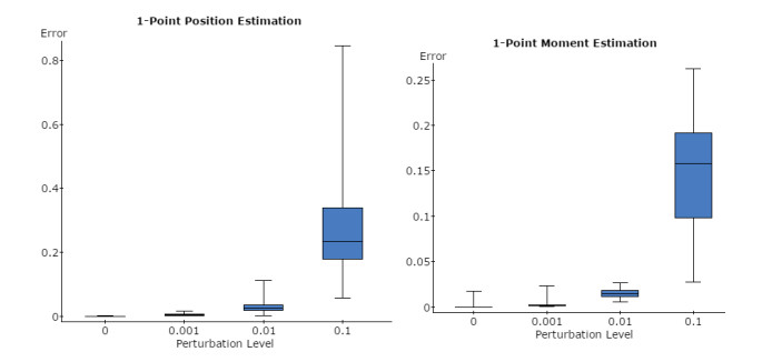
In this paper we study a harmonic function method for dipolar source reconstruction, and implemented the numerical simulations. We propose a new error estimate and provide a rigorous proof of the estimate. Then, we validate our method in computer-simulated data and study its numerical stability in different noise levels. It is shown that the harmonic function method can be used to quickly and accurately locate the active regions in EEG source reconstruction.
Citation: Hongguang Xi, Jianzhong Su. A harmonic function method for EEG source reconstruction[J]. Electronic Research Archive, 2022, 30(2): 492-514. doi: 10.3934/era.2022026
In this paper we study a harmonic function method for dipolar source reconstruction, and implemented the numerical simulations. We propose a new error estimate and provide a rigorous proof of the estimate. Then, we validate our method in computer-simulated data and study its numerical stability in different noise levels. It is shown that the harmonic function method can be used to quickly and accurately locate the active regions in EEG source reconstruction.

| [1] |
N. K. Logothetis, What we can do and what we cannot do with fMRI, Nature, 453 (2008), 869–878. https://doi.org/10.1038/nature06976 doi: 10.1038/nature06976

|
| [2] |
B. He, J. Lian, High-resolution spatio-temporal functional neuroimaging of brain activity, Crit. Rev. Biomed. Eng., 30 (2002), 283–306. https://doi.org/10.1615/CritRevBiomedEng.v30.i456.30 doi: 10.1615/CritRevBiomedEng.v30.i456.30
|
| [3] | P. L. Nunez, Electric Fields of the Brain: The Neurophysics of EEG, Oxford University Press, 1981. |
| [4] |
R. Grave de Peralta Menendez, S. L. Gonzalez Andino, S. Morand, C. M. Michel, T. Landis, Imaging the electrical activity of the brain: ELECTRA, Hum. Brain Mapp., 9 (2000), 1–12. https://doi.org/10.1002/(SICI)10970193(2000)9:1<1::AIDHBM1>3.0.CO;2# doi: 10.1002/(SICI)10970193(2000)9:1<1::AIDHBM1>3.0.CO;2#
|
| [5] | C. M. Michel, M. M. Murray, G. Lantz, S. Gonzalez, L. Spinelli, R. Grave de Peralta, EEG source imaging, Clin. Neurophysiol., 115 (2004), 2195–2222. https://doi.org/10.1016/j.clinph.2004.06.001 |
| [6] |
A. Hunter, B. Crouch, N. Webster, B. Platt, Delirium screening in the intensive care unit using emerging qeeg techniques: A pilot study, AIMS Neurosci., 7 (2020), 1–16. https://doi.org/10.3934/Neuroscience.2020001 doi: 10.3934/Neuroscience.2020001
|
| [7] |
G. V. Portnova, O. Ivanova, E. V. Proskurnina, Effects of eeg examination and aba-therapy on resting-state eeg in children with low-functioning autism, AIMS Neurosci., 7 (2020), 153–167. https://doi.org/10.3934/Neuroscience.2020011 doi: 10.3934/Neuroscience.2020011
|
| [8] |
R. Grech, T. Cassar, J. Muscat, K. P. Camilleri, S. G. Fabri, M. Zervakis, et al., Review on solving the inverse problem in EEG source analysis, J. NeuroEng. Rehabilitation, 5 (2008), 25. https://doi.org/10.1186/1743-0003-5-25 doi: 10.1186/1743-0003-5-25
|
| [9] | V. Isakov, Inverse Problems for Partial Differential Equations, Springer, 2nd edition, 2005. |
| [10] |
S. Vessella, Locations and strengths of point sources: stability estimates, Inverse Probl., 8 (1992), 911. https://doi.org/10.1088/0266-5611/8/6/008 doi: 10.1088/0266-5611/8/6/008
|
| [11] |
R. M. Leahy, J. C. Mosher, M. E. Spencer, M. X. Huang, J. D. Lewine, A study of dipole localization accuracy for meg and eeg using a human skull phantom, Electroencephalogr. clin. neurophysiol., 107 (1998), 159–173. https://doi.org/10.1016/S0013-4694(98)00057-1 doi: 10.1016/S0013-4694(98)00057-1
|
| [12] |
A. El Badia, T. Ha-Duong, An inverse source problem in potential analysis, Inverse Probl., 16 (2000), 651–663. https://doi.org/10.1088/0266-5611/16/3/308 doi: 10.1088/0266-5611/16/3/308
|
| [13] | M. Chafik, A. El Badia, T. Ha-Duong, On some inverse eeg problems, Inverse Probl. Eng. Mech. II, pages 537–544, 2000. https://doi.org/10.1016/B978-008043693-7/50129-X |
| [14] |
T. Nara, S. Ando, A projective method for an inverse source problem of the poisson equation, Inverse Probl., 19 (2003), 355–369. https://doi.org/10.1088/0266-5611/19/2/307 doi: 10.1088/0266-5611/19/2/307
|
| [15] |
H. Kang, H. Lee, Identification of simple poles via boundary measurements and an application of eit, Inverse Probl., 20 (2004), 1853. https://doi.org/10.1088/0266-5611/20/6/010 doi: 10.1088/0266-5611/20/6/010
|
| [16] |
A. El Badia, Inverse source problem in an anisotropic medium by boundary measurements, Inverse Probl., 21 (2005), 1487. https://doi.org/10.1088/0266-5611/21/5/001 doi: 10.1088/0266-5611/21/5/001
|
| [17] |
L. Baratchart, A. Ben Abda, F. Ben Hassen, J. Leblond, Recovery of pointwise sources or small inclusions in 2d domains and rational approximation, Inverse Probl., 21 (2005), 51. https://doi.org/10.1088/0266-5611/21/1/005 doi: 10.1088/0266-5611/21/1/005
|
| [18] |
Y. S. Chung, S. Y. Chung, Identification of the combination of monopolar and dipolar sources for elliptic equations, Inverse Probl., 25 (2009), 085006. https://doi.org/10.1088/0266-5611/25/8/085006 doi: 10.1088/0266-5611/25/8/085006
|
| [19] | D. Kandaswamy, T. Blu, D. van de Ville, Analytic sensing: Noniterative retrieval of point sources from boundary measurements, SIAM J. Sci. Comput., 31 (2009), 3179–3194. https://doi.org/10.1137/080712829 |
| [20] |
T. Nara, S. Ando, Direct localization of poles of a meromorphic function from measurements on an incomplete boundary, Inverse Probl., 26 (2010), 015011. https://doi.org/10.1088/0266-5611/26/1/015011 doi: 10.1088/0266-5611/26/1/015011
|
| [21] |
A. El Badia, T. Nara, An inverse source problem for helmholtz's equation from the cauchy data with a single wave number, Inverse Probl., 27 (2011), 105001. https://doi.org/10.1088/0266-5611/27/10/105001 doi: 10.1088/0266-5611/27/10/105001
|
| [22] |
M. Clerc, J. Leblond, J.-P. Marmorat, T. Papadopoulo, Source localization using rational approximation on plane sections, Inverse Probl., 28 (2012), 055018. https://doi.org/10.1088/0266-5611/28/5/055018 doi: 10.1088/0266-5611/28/5/055018
|
| [23] |
R. Mdimagh, I.Ben Saad, Stability estimates for point sources identification problem using reciprocity gap concept via the helmholtz equation, Appl. Math. Model., 40 (2016), 7844–7861. https://doi.org/10.1016/j.apm.2016.03.024 doi: 10.1016/j.apm.2016.03.024
|
| [24] | J. Vorwerk, Ü. Aydin, C. H. Wolters, C. R. Butson, Influence of head tissue conductivity uncertainties on eeg dipole reconstruction, Front Neurosci., 13 (2019), PMCID: PMC6558618. https://doi.org/10.3389/fnins.2019.00531 |
| [25] |
M. Rubega, M. Carboni, M. Seeber, D. Pascucci, S. Tourbier, G. Toscano, et al., Estimating eeg source dipole orientation based on singular-value decomposition for connectivity analysis, Brain topogr., 32 (2019), 704–719. https://doi.org/10.1007/s10548-018-0691-2 doi: 10.1007/s10548-018-0691-2
|
| [26] | M. S. Hämäläinen, R. J. Ilmoniemi, Interpreting magnetic fields of the brain: minimum norm estimates, Med. Biol. Eng. & Comput., 32 (1994), 35–42. https://doi.org/10.1007/BF02512476 |
| [27] | R. D. Pascual-Marqui, Review of methods for solving the eeg inverse problem, Int. J. Bioelectromagn., 1 (1999), 75–86, 1999. |
| [28] | S. Baillet, Toward functional brain imaging of cortical electrophysiology markovian models for magneto and electroencephalogram source estimation and experimental assessments, Orsay, France, 1998. |
| [29] | S. Baillet, J. C. Mosher, R. M. Leahy, Electromagnetic brain mapping, IEEE Signal Process. Mag., 18 (2001), 14–30. https://doi.org/10.1109/79.962275 |
| [30] | J. C. Mosher, P. S. Lewis, R. M. Leahy, Multiple dipole modeling and localization from spatio-temporal MEG data, IEEE Trans. Biomed. Eng., 39 (1992), 541–557. https://doi.org/10.1109/10.141192 |
| [31] |
P. A. Muñoz Gutiérrez, E. Giraldo, M. Bueno-López, M. Molinas, Localization of active brain sources from eeg signals using empirical mode decomposition: a comparative study, Front. Integrat. Neurosci., 2 (2018), 55. https://doi.org/10.3389/fnint.2018.00055 doi: 10.3389/fnint.2018.00055
|
| [32] |
C. Kaur, P. Singh, S. Sahni, Electroencephalography-based source localization for depression using standardized low resolution brain electromagnetic tomography-variational mode decomposition technique, Eur. Neurol., 81 (2019), 63–75. https://doi.org/10.1159/000500414 doi: 10.1159/000500414
|
| [33] | V. P. Oikonomou, I. Kompatsiaris, A novel bayesian approach for eeg source localization, Comput. Intell. Neurosci., 2020. https://doi.org/10.1155/2020/8837954 |
| [34] |
S. Andrieux, A. Ben Abda, H.D. Bui, Reciprocity principle and crack identification, Inverse Probl., 15 (1999), 59. https://doi.org/10.1088/0266-5611/15/1/010 doi: 10.1088/0266-5611/15/1/010
|
| [35] |
H. Azizollahi, M. Darbas, M. M. Diallo, A. El Badia, S. Lohrengel, EEG in neonates: Forward modeling and sensitivity analysis with respect to variations of the conductivity, Math. Biosci. Eng., 15 (2018), 905–932. https://doi.org/10.3934/mbe.2018041 doi: 10.3934/mbe.2018041
|


Figures(7) / Tables(1)
Hongguang Xi, Jianzhong Su. A harmonic function method for EEG source reconstruction[J]. Electronic Research Archive, 2022, 30(2): 492-514. doi: 10.3934/era.2022026


 DownLoad: