An adaptive edge finite element method for the Maxwell's equations in metamaterials

Hao Wang; Wei Yang; Yunqing Huang; Hao Wang; Wei Yang; Yunqing Huang

doi:10.3934/era.2020051

Electronic Research Archive

2020, Volume 28, Issue 2: 961-976. doi: 10.3934/era.2020051

Previous Article Next Article

Special Issues

An adaptive edge finite element method for the Maxwell's equations in metamaterials

Hao Wang ^{1
,},
Wei Yang ^{1
,},
Yunqing Huang ^{2
,}

1.
Hunan Key Laboratory for Computation and Simulation in Science and Engineering, School of Mathematics and Computational Science, Xiangtan University, Xiangtan 411105, Hunan, China
2.
Key Laboratory of Intelligent Computing & Information Processing of Ministry of Education, School of Mathematics and Computational Science, Xiangtan University, Xiangtan 411105, Hunan, China

Received: 01 February 2020 Revised: 01 April 2020
78M10, 65N30

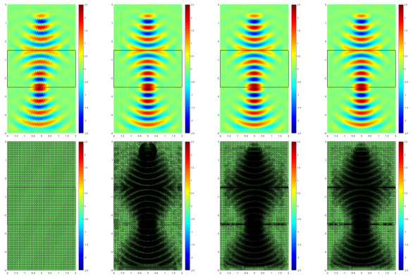
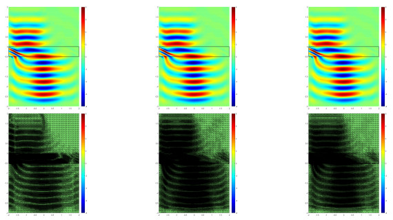
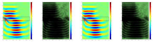
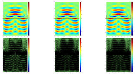
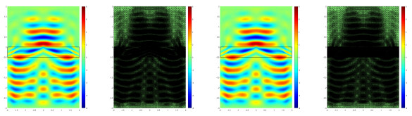
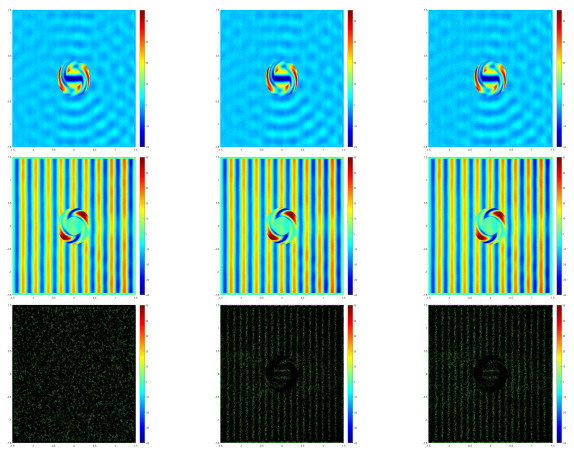
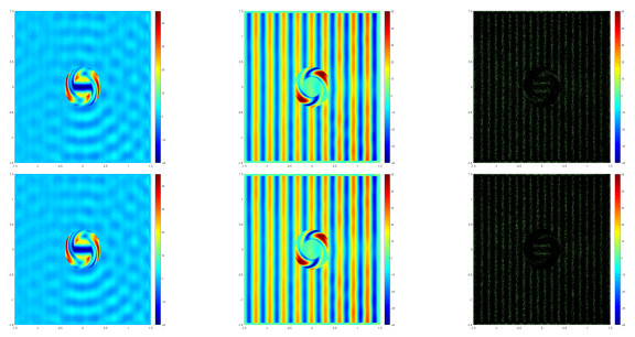
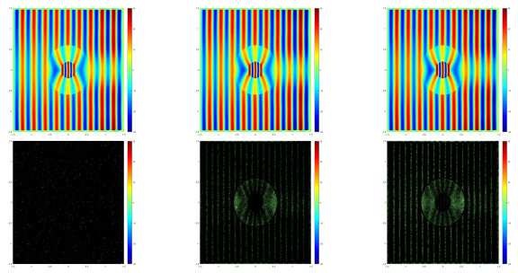
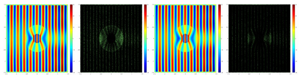
In this paper, we study an adaptive edge finite element method for time-harmonic Maxwell's equations in metamaterials. A-posteriori error estimators based on the recovery type and residual type are proposed, respectively. Based on our a-posteriori error estimators, the adaptive edge finite element method is designed and applied to simulate the backward wave propagation, electromagnetic splitter, rotator, concentrator and cloak devices. Numerical examples are presented to illustrate the reliability and efficiency of the proposed a-posteriori error estimations for the adaptive method.
- Maxwell's equations,
- wave source terms,
- a-posteriori error estimator,
- adaptive edge finite element method,
- metamaterial media
Citation: Hao Wang, Wei Yang, Yunqing Huang. An adaptive edge finite element method for the Maxwell's equations in metamaterials[J]. Electronic Research Archive, 2020, 28(2): 961-976. doi: 10.3934/era.2020051

Related Papers:

Abstract

In this paper, we study an adaptive edge finite element method for time-harmonic Maxwell's equations in metamaterials. A-posteriori error estimators based on the recovery type and residual type are proposed, respectively. Based on our a-posteriori error estimators, the adaptive edge finite element method is designed and applied to simulate the backward wave propagation, electromagnetic splitter, rotator, concentrator and cloak devices. Numerical examples are presented to illustrate the reliability and efficiency of the proposed a-posteriori error estimations for the adaptive method.

References

[1]	Plasmon resonance with finite frequencies: A validation of the quasi-static approximation for diametrically small inclusions. SIAM J. Appl. Math. (2016) 76: 731-749.
[2]	Nearly cloaking the full Maxwell equations: Cloaking active contents with general conducting layers. J. Math. Pures. Appl. (9) (2014) 101: 716-733.
[3]	A perfectly matched layer for the absorption of electromagnetic waves. J. Comput. Phys. (1994) 114: 185-200.
[4]	Localization and geometrization in plasmon resonances and geometric structures of Neumann-Poincaré eigenfunctions. ESAIM Math. Model. Numer. Anal. (2020) 54: 957-976.
[5]	Analysis of a Cartesian PML approximation to the three dimensional electromagnetic wave scattering problem. Int. J. Numer. Anal. Model. (2012) 9: 543-561.
[6]	An adaptive $P_1$ finite element method for two-dimensional Maxwell's equations. J. Sci. Comput. (2013) 55: 738-754.
[7]	An adaptive $P_1$ finite element method for two-dimensional transverse magnetic time harmonic Maxwell's equations with general material properties and general boundary conditions. J. Sci. Comput. (2016) 68: 848-863.
[8]	A recovery-based a posteriori error estimator for $H$(curl) interface problems. Comput. Methods. Appl. Mech. Engrg. (2015) 296: 169-195.
[9]	Recovery-based error estimators for interface problems: Mixed and nonconforming finite elements. SIAM J. Numer. Anal. (2010) 48: 30-52.
[10]	Flux recovery and a posteriori error estimators: Conforming elements for scalar elliptic equations. SIAM J. Numer. Anal. (2010) 48: 578-602.
[11]	Multigrid methods for two-dimensional Maxwell's equations on graded meshes. J. Comput. Appl. Math. (2014) 255: 231-247.
[12]	Full and partial cloaking in electromagnetic scattering. Arch. Ration. Mech. Anal. (2017) 223: 265-299.
[13]	A convergent adaptive algorithm for Poisson's equation. SIAM J. Numer. Anal. (1996) 33: 1106-1124.
[14]	Y. Hao and R. Mittra, FDTD modeling of metamaterials: Theory and applications, Artech. House., (2008).
[15]	B. He, W. Yang and H. Wang, Convergence analysis of adaptive edge finite element method for variable coefficient time-harmonic Maxwell's equations, J. Comput. Appl. Math., 376 (2020), 16pp. doi: 10.1016/j.cam.2020.112860
[16]	The averaging technique for superconvergence: Verification and application of 2D edge elements to Maxwell's equations in metamaterials. Comput. Methods Appl. Mech. Engrg. (2013) 255: 121-132.
[17]	Interior penalty DG methods for Maxwell's equations in dispersive media. J. Comput. Phys. (2011) 230: 4559-4570.
[18]	Y. Huang, J. Li and W. Yang, Modeling backward wave propagation in metamaterials by the finite element time-domain method, SIAM J. Sci. Comput., 35 (2013), B248–B274. doi: 10.1137/120869869
[19]	The superconvergent cluster recovery method. J. Sci. Comput. (2010) 44: 301-322.
[20]	On quasi-static cloaking due to anomalous localized resonance in $\mathbb{R}^{3}$. SIAM J. Appl. Math. (2015) 75: 1245-1260.
[21]	Analysis of electromagnetic scattering from plasmonic inclusions beyond the quasi-static approximation and applications. ESAIM Math. Model. Numer. Anal. (2019) 53: 1351-1371.
[22]	Analysis and application of the nodal discontinuous Galerkin method for wave propagation in metamaterials. J. Comput. Phys. (2014) 258: 915-930.
[23]	An adaptive edge finite element method for electromagnetic cloaking simulation. J. Comput. Phys. (2013) 249: 216-232.
[24]	H. Liu, Virtual reshaping and invisibility in obstacle scattering, Inverse Problems, 25 (2009), 16pp. doi: 10.1088/0266-5611/25/4/045006
[25]	(2003) Finite Element Methods for Maxwell's Equations.Oxford University Press.
[26]	A posteriori error estimates based on the polynomial preserving recovery. SIAM J. Numer. Anal. (2004) 42: 1780-1800.
[27]	Hybridizable discontinuous Galerkin methods for the time-harmonic Maxwell's equations. J. Comput. Phys. (2011) 230: 7151-7175.
[28]	Controlling electromagnetic fields. Science (2006) 312: 1780-1782.
[29]	Adjoint recovery of superconvergent functionals from PDE approximations. SIAM. Rev. (2000) 42: 247-264.
[30]	A. Taflove and S. C. Hagness, Computational Electrodynamics: The Finite-Difference Time-Domain Method, Artech House, Inc., Boston, MA, 2000.
[31]	Adaptive finite element method for the sound wave problems in two kinds of media. Comput. Math. Appl. (2020) 79: 789-801.
[32]	D. H. Werner and D.-H. Kwon, Transformation Electromagnetics and Metamaterials. Fundamental Principles and Applications, Springer-Verlag, London, 2014. doi: 10.1007/978-1-4471-4996-5
[33]	Developing a time-domain finite element method for the Lorentz metamaterial model and applications. J. Sci. Comput. (2016) 68: 438-463.
[34]	Modeling and analysis of the optical black hole in metamaterials by the finite element time-domain method. Comput. Methods Appl. Mech. Engrg. (2016) 304: 501-520.
[35]	Mathematical analysis and finite element time domain simulation of arbitrary star-shaped electromagnetic cloaks. SIAM J. Numer. Anal. (2018) 56: 136-159.
[36]	Developing finite element methods for simulating transformation optics devices with metamaterials. Commun. Comput. Phys. (2019) 25: 135-154.
[37]	The superconvergence patch recovery (SPR) and adaptive finite element refinement. Comput. Methods. Appl. Mech. Engrg. (1992) 101: 207-224.

Reader Comments

your name:*

Email:*
© 2020 the Author(s), licensee AIMS Press. This is an open access article distributed under the terms of the Creative Commons Attribution License (http://creativecommons.org/licenses/by/4.0)