The effect of biochar on hydrologic fluxes was estimated using a single hillslope version of a gridded soil moisture routing (SMR) model. Five grid cells were aligned linearly with varied slopes to simulate a small undulating hillslope with or without a restrictive layer beneath the soil profile. Biochar amendments (redwood sawdust and wheat straw biochar) at concentrations of 0%, 4%, and 7% were applied to the topmost grid-cell by mass of dry soil. Simulated streamflow hydrographs for restricted and non-restricted soil profiles were manually calibrated with measured Palouse River streamflow data. Evapotranspiration, percolation, lateral flow, baseflow, and streamflow were all modeled yearly. Two generally reported field capacities (FC) in literature at −6 and −33 kPa were considered to assess the effect of biochar. Field capacity considered at −6 kPa corresponds to higher moisture content, and hence higher moisture storage capacity between FC and permanent wilting point than at −33 kPa. At −6 kPa FC, biochar effectively increased evapotranspiration and reduced the lateral flow of the system. Increased soil porosity from biochar amendment enhanced the water holding capacity of the soil and plant available water. These mechanisms impacted the streamflow generated from the system indicating positive outcomes from biochar amendment in both restricted and non-restricted soil profiles. Biochar amendment showed an order of magnitude smaller effects with −33 kPa FC compared to −6 kPa FC; the increased porosity appeared to be less influential at lower field capacity values. Additionally, the results showed that the over-application of coarse biochar might negatively affect retaining soil moisture. These findings point to positive results for using biochar as a water management strategy if applied less than 7% in this study, but further exploration is needed to find the optimum level of biochar with different biochar and soil properties.
Citation: Adam O'Keeffe, Erin Brooks, Chad Dunkel, Dev S. Shrestha. Soil moisture routing modeling of targeted biochar amendment in undulating topographies: an analysis of biochar's effects on streamflow[J]. AIMS Environmental Science, 2023, 10(4): 529-546. doi: 10.3934/environsci.2023030
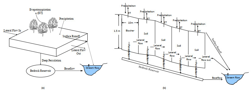
The effect of biochar on hydrologic fluxes was estimated using a single hillslope version of a gridded soil moisture routing (SMR) model. Five grid cells were aligned linearly with varied slopes to simulate a small undulating hillslope with or without a restrictive layer beneath the soil profile. Biochar amendments (redwood sawdust and wheat straw biochar) at concentrations of 0%, 4%, and 7% were applied to the topmost grid-cell by mass of dry soil. Simulated streamflow hydrographs for restricted and non-restricted soil profiles were manually calibrated with measured Palouse River streamflow data. Evapotranspiration, percolation, lateral flow, baseflow, and streamflow were all modeled yearly. Two generally reported field capacities (FC) in literature at −6 and −33 kPa were considered to assess the effect of biochar. Field capacity considered at −6 kPa corresponds to higher moisture content, and hence higher moisture storage capacity between FC and permanent wilting point than at −33 kPa. At −6 kPa FC, biochar effectively increased evapotranspiration and reduced the lateral flow of the system. Increased soil porosity from biochar amendment enhanced the water holding capacity of the soil and plant available water. These mechanisms impacted the streamflow generated from the system indicating positive outcomes from biochar amendment in both restricted and non-restricted soil profiles. Biochar amendment showed an order of magnitude smaller effects with −33 kPa FC compared to −6 kPa FC; the increased porosity appeared to be less influential at lower field capacity values. Additionally, the results showed that the over-application of coarse biochar might negatively affect retaining soil moisture. These findings point to positive results for using biochar as a water management strategy if applied less than 7% in this study, but further exploration is needed to find the optimum level of biochar with different biochar and soil properties.

| [1] | Hall M, Young D L, Walker D J (1999) Agriculture in the Palouse, a Portrait of Diversity. Moscow, ID: BUL 794. University of Idaho. |
| [2] | Hartmans MA, Michalson EL (1998) Evaluating the Economic & Environmental Impacts of Farming Practices on the Palouse Using PLANETOR. Moscow, ID: Agricultural Experiment & UI Extension Publications, University of Idaho. |
| [3] |
Beven KJ, Kirkby MJ (1979) A physically based, variable contributing area model of basin hydrology / Un modèle à base physique de zone d'appel variable de l'hydrologie du bassin versant. Hydrolog Sci Bull 24: 43–69. doi: https://doi.org/10.1080/02626667909491834. doi: 10.1080/02626667909491834

|
| [4] |
Wilson DJ, Western AW, Grayson RB (2005) A terrain and data-based method for generating the spatial distribution of soil moisture. Adv Water Resour 28: 43–54. doi: https://doi.org/10.1016/j.advwatres.2004.09.007. doi: 10.1016/j.advwatres.2004.09.007
|
| [5] |
Schlegel AJ, Assefa Y, Haag LA, et al. (2017) Yield and Soil Water in Three Dryland Wheat and Grain Sorghum Rotations. Agron J 109: 227–38. doi: https://doi.org/10.2134/agronj2016.07.0387. doi: 10.2134/agronj2016.07.0387
|
| [6] |
Fuentes JP, Flury M, Huggins DR, et al. (2003) Soil water and nitrogen dynamics in dryland cropping systems of Washington State, USA. Soil Till Res USA 71: 33–47. doi: https://doi.org/10.1016/S0167-1987(02)00161-7. doi: 10.1016/S0167-1987(02)00161-7
|
| [7] |
Jin K, Cornelis WM, Schiettecatte W, et al. (2007) Effects of different management practices on the soil–water balance and crop yield for improved dryland farming in the Chinese Loess Plateau. Soil Till Res 96: 131–44. doi: https://doi.org/10.1016/j.still.2007.05.002. doi: 10.1016/j.still.2007.05.002
|
| [8] |
Kühling I, Redozubov D, Broll G, et al. (2017) Impact of tillage, seeding rate and seeding depth on soil moisture and dryland spring wheat yield in Western Siberia. Soil Till Res 170: 43–52. doi: https://doi.org/10.1016/j.still.2017.02.009. doi: 10.1016/j.still.2017.02.009
|
| [9] |
Brown M, Heinse R, Johnson-Maynard J, et al. (2021) Time-lapse mapping of crop and tillage interactions with soil water using electromagnetic induction. Vadose Zone J 20: e20097. doi: https://doi.org/10.1002/vzj2.20097. doi: 10.1002/vzj2.20097
|
| [10] |
Eagleson PS (1978) Climate, soil, and vegetation: 1. Introduction to water balance dynamics. Water Resour Res 14: 705–12. doi: https://doi.org/10.1029/WR014i005p00705. doi: 10.1029/WR014i005p00705
|
| [11] |
Burt TP, Butcher DP (1985) Topographic controls of soil moisture distributions. J Soil Sci 36: 469–486. doi: https://doi.org/10.1111/j.1365-2389.1985.tb00351.x. doi: 10.1111/j.1365-2389.1985.tb00351.x
|
| [12] |
Sheets KR, Hendrickx JMH (1995) Noninvasive Soil Water Content Measurement Using Electromagnetic Induction. Water Resour Res 31: 2401–2419. doi: https://doi.org/10.1029/95WR01949. doi: 10.1029/95WR01949
|
| [13] | Kaiser VG (1967) Soil erosion and wheat yields in Whitman County, Washington. Northwest Sci. Soil erosion and wheat yields in Whitman County, Washington 41: 6. |
| [14] | USDA (1978) Palouse Cooperative River Basin Study. Washington D.C.: 1978. Report No.: 719153. |
| [15] | Brooks ES, Boll J, McDaniel PA (2012) Chapter 10 - Hydropedology in Seasonally Dry Landscapes: The Palouse Region of the Pacific Northwest USA. In: Lin H, editor. Hydropedology. Boston: Academic Press. p. 329–350. |
| [16] |
Brooks ES, Boll J, McDaniel PA (2004) A hillslope-scale experiment to measure lateral saturated hydraulic conductivity. Water Resour Res 40. doi: https://doi.org/10.1029/2003WR002858. doi: 10.1029/2003WR002858
|
| [17] |
McDaniel PA, Gabehart RW, Falen AL, et al. (2001) Perched Water Tables on Argixeroll and Fragixeralf Hillslopes. Soil Sci Soc Am J s 65: 805–810. doi: https://doi.org/10.2136/sssaj2001.653805x. doi: 10.2136/sssaj2001.653805x
|
| [18] |
McDaniel PA, Regan MP, Brooks E, et al. (2008) Linking fragipans, perched water tables, and catchment-scale hydrological processes. Catena 73: 166–173. doi: https://doi.org/10.1016/j.catena.2007.05.011. doi: 10.1016/j.catena.2007.05.011
|
| [19] |
Western AW, Grayson RB, Blöschl G (2002) Scaling of Soil Moisture: A Hydrologic Perspective. Annu Rev Earth Pl Sc 30: 149–180. doi: https://doi.org/10.1146/annurev.earth.30.091201.140434. doi: 10.1146/annurev.earth.30.091201.140434
|
| [20] |
Zhu Q, Lin H, Doolittle J (2010) Repeated Electromagnetic Induction Surveys for Determining Subsurface Hydrologic Dynamics in an Agricultural Landscape. Soil Sci Soc Am J 74: 1750–1762. doi: https://doi.org/10.2136/sssaj2010.0055. doi: 10.2136/sssaj2010.0055
|
| [21] |
Corwin DL, Lesch SM (2003) Application of Soil Electrical Conductivity to Precision Agriculture. Agron J 95: 455–471. doi: https://doi.org/10.2134/agronj2003.4550. doi: 10.2134/agronj2003.4550
|
| [22] |
Corwin DL, Lesch SM (2005) Apparent soil electrical conductivity measurements in agriculture. Comput Electron Agr 46: 11–43. doi: https://doi.org/10.1016/j.compag.2004.10.005. doi: 10.1016/j.compag.2004.10.005
|
| [23] | Weddell B, Brown T, Borrelli K (2017) Chapter 8: Precision Agriculture. In: Yorgey G, Kruger C, editors. Advances in Dryland Farming in the Inland Pacific Northwest. Pullman, Washington: Washington State University. |
| [24] | O'Keeffe AL, Shrestha D, Brooks E, et al. (2020) Modeling Palouse hills to quantify moisture redistribution from the selective non-uniform application of biochar. SABE Annual International Meeting; Omaha, Nebraska: American Society of Agricultural and Biological Engineers. p. pages 1–12. |
| [25] |
Yang C, Peterson CL, Shropshire GJ, et al. (1998) Spatial variability of field topography and wheat yield in the Palouse region of the Pacific Northwest. T ASAE 41: 17–27. doi: https://doi.org/10.13031/2013.17147. doi: 10.13031/2013.17147
|
| [26] | Lehmann J, Joseph S (2009) Chapter 1- Biochar for Environmental Management: An Introduction. Biochar for Environmental Management: Routledge. |
| [27] | Masiello CA, Dugan B, Brewer CE, et al. (2019) Biochar effects on soil hydrology. Biochar for Environmental Management 2nd Edition. |
| [28] |
Aller D, Rathke S, Laird D, et al. (2017) Impacts of fresh and aged biochars on plant available water and water use efficiency. Geoderma 307: 114–121. doi: https://doi.org/10.1016/j.geoderma.2017.08.007. doi: 10.1016/j.geoderma.2017.08.007
|
| [29] |
Dokoohaki H, Miguez FE, Laird D, et al. (2017) Assessing the Biochar Effects on Selected Physical Properties of a Sandy Soil: An Analytical Approach. Commun Soil Sci Plan 48: 1387–1398. doi: https://doi.org/10.1080/00103624.2017.1358742. doi: 10.1080/00103624.2017.1358742
|
| [30] | Joint Research C, Institute for E, Sustainability, Bastos A, Verheijen F, Jeffery S (2010) Biochar application to soils: a critical scientific review of effects on soil properties, processes and functions: Publications Office. |
| [31] |
Razzaghi F, Obour PB, Arthur E (2020) Does biochar improve soil water retention? A systematic review and meta-analysis. Geoderma 361: 114055. doi: https://doi.org/10.1016/j.geoderma.2019.114055. doi: 10.1016/j.geoderma.2019.114055
|
| [32] | McCool D, Huggins D, Saxton K, et al. (2001) Factors affecting agricultural sustainability in the Pacific Northwest, USA: An overview.. In: Mohtar RH, Steinhardt GC, Stott DE, editors. Sustaining the Global Farm: Selected Papers from the 10th International Soil Conservation Organization Meeting. West Lafayette: Purdue University. p. 255–260. |
| [33] | NRCS (2022) Keys to soil taxonomy. 13th ed: United States Department of Agriculture, Natural Resources Conservation Service. |
| [34] | NRCS (2023) Web Site for Official Soil Series Descriptions and Series Classification Washington D.C.: U.S. Department of Agriculture, National Cooperative Soil Survey. Available from: https://soilseries.sc.egov.usda.gov/OSD_Docs/P/PALOUSE.html. |
| [35] |
Frankenberger JR, Brooks ES, Walter MT, et al. (1999) A GIS-based variable source area hydrology model. Hydrol Process 13: 805–822. doi: https://doi.org/10.1002/(SICI)1099-1085(19990430)13:6<805::AID-HYP754>3.0.CO;2-M. doi: 10.1002/(SICI)1099-1085(19990430)13:6<805::AID-HYP754>3.0.CO;2-M
|
| [36] |
Brooks ES, Boll J, McDaniel PA (2007) Distributed and integrated response of a geographic information system-based hydrologic model in the eastern Palouse region, Idaho. Hydrol Process 21: 110–122. doi: https://doi.org/10.1002/hyp.6230. doi: 10.1002/hyp.6230
|
| [37] |
Johnson MS, Coon WF, Mehta VK, et al. (2003) Application of two hydrologic models with different runoff mechanisms to a hillslope dominated watershed in the northeastern US: a comparison of HSPF and SMR. J Hydrol 284: 57–76. doi: https://doi.org/10.1016/j.jhydrol.2003.07.005. doi: 10.1016/j.jhydrol.2003.07.005
|
| [38] | Allen R (2013) Ref-ET: Reference Evapotranspiration Calculation Software for FAO and ASCE Standardized Equations Kimberly, Idaho: University of Idaho; [cited 2023 May, 28]. Version 3.1: [Available from: https://www.webpages.uidaho.edu/ce325bae355/references/manual_prn.pdf. |
| [39] | Allen RG, Pereira LS, Raes D, et al. (1998) FAO Irrigation & drainage Paper No. 56: Crop evapotranspiration (guidelines for computing crop water requirements).Rome, Italy: FAO - Food and Agriculture Organization of the United Nations. |
| [40] | NDAWN (2023) Wheat Growth Stage Prediction Using Growing Degree Days (GDD) Fargo, North Dakota: North Dakota Agricultural Weather Network; [cited 2023 May, 28]. Available from: https://ndawn.ndsu.nodak.edu/help-wheat-growing-degree-days.html. |
| [41] |
O'Keeffe A, Shrestha D, Dunkel C, et al. (2023) Modeling moisture redistribution from selective non-uniform application of biochar on Palouse hills. Agr Water Manage 277. doi: https://doi.org/10.1016/j.agwat.2022.108026. doi: 10.1016/j.agwat.2022.108026
|
| [42] |
Schindler U, Durner W, von Unold G, et al. (2010) Evaporation Method for Measuring Unsaturated Hydraulic Properties of Soils: Extending the Measurement Range. Soil Sci Soc Am J 74: 1071–1083. doi: https://doi.org/10.2136/sssaj2008.0358. doi: 10.2136/sssaj2008.0358
|
| [43] |
Van Genuchten M (1980) A Closed-form Equation for Predicting the Hydraulic Conductivity of Unsaturated Soils Soil Sci Soc Am J 44. doi: https://doi.org/10.2136/sssaj1980.03615995004400050002x. doi: 10.2136/sssaj1980.03615995004400050002x
|
| [44] | de Oliveira RA, Ramos MM, de Aquino LA (2015) Chapter 8 - Irrigation Management. In: Santos F, Borém A, Caldas C, editors. Sugarcane. San Diego: Academic Press. p. 161–183. |
| [45] |
de Jong van Lier Q (2017) Field capacity, a valid upper limit of crop available water? Agr Water Manage 193: 214–220. doi: https://doi.org/10.1016/j.agwat.2017.08.017. doi: 10.1016/j.agwat.2017.08.017
|
| [46] | NRCS (2023) National Water and Climate Center Data: United States Department of Agriculture, Natural Resources Conservation Service. Available from: https://wcc.sc.egov.usda.gov/nwcc/site?sitenum = 989. |
| [47] |
Moriasi DN, Arnold JG, Van Liew MW, et al. (2007) Model Evaluation Guidelines for Systematic Quantification of Accuracy in Watershed Simulations. T ASABE 50: 885–900. doi: https://doi.org/10.13031/2013.23153. doi: 10.13031/2013.23153
|
| [48] |
Devak M, Dhanya CT (2017) Sensitivity analysis of hydrological models: review and way forward. J Water Clim Change 8: 557–575. doi: https://doi.org/10.2166/wcc.2017.149. doi: 10.2166/wcc.2017.149
|
| [49] | Koenig RT (2005) Dryland Winter Wheat : Eastern Washington Nutrient Management Guide. Department of Crop and Soil Sciences, Washington State University, Pullman. |
| [50] |
Grayson RB, Moore ID, McMahon TA (1992) Physically based hydrologic modeling: 2. Is the concept realistic? Water Resour Res 28: 2659–2666. doi: https://doi.org/10.1029/92WR01259. doi: 10.1029/92WR01259
|


Figures(4) / Tables(4)

Adam O'Keeffe, Erin Brooks, Chad Dunkel, Dev S. Shrestha. Soil moisture routing modeling of targeted biochar amendment in undulating topographies: an analysis of biochar's effects on streamflow[J]. AIMS Environmental Science, 2023, 10(4): 529-546. doi: 10.3934/environsci.2023030


 DownLoad: