Spatiotemporal analysis of drought occurrence in the Ouergha catchment, Morocco

Kaoutar MOUNIR; Isabelle LA JEUNESSE; Haykel SELLAMI; Abdessalam ELKHANCHOUFI; Kaoutar MOUNIR; Isabelle LA JEUNESSE; Haykel SELLAMI; Abdessalam ELKHANCHOUFI

doi:10.3934/environsci.2023023

AIMS Environmental Science

2023, Volume 10, Issue 3: 398-423. doi: 10.3934/environsci.2023023

Previous Article Next Article

Research article

Spatiotemporal analysis of drought occurrence in the Ouergha catchment, Morocco

1.
University Sidi Mohamed Ben Abdallah of Fez, CED ST LGE2D, Fez, Morocco
2.
University of Tours, UMR CNRS 7324 Citeres, 33 allée Ferdinand de Lesseps, 37204 Tours cedex 3, France
3.
Centre for Water Research and Technology, EcoPark BorjCedria, Soliman, Tunisia
4.
UMR 7300 ESPACE, Université Côte d'Azur, Mediterranean Institute of Environmental Risk and Sustainable Development, Nice Meridia Technopole, 9, Rue Julien Lauprêtre, 06200 Nice, France

Received: 19 November 2022 Revised: 03 March 2023 Accepted: 22 March 2023 Published: 04 May 2023

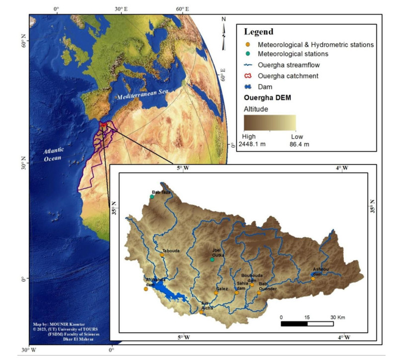
Although the spatiotemporal characterization of droughts is a key step in the design and implementation of practical measures to mitigate their impacts, it is hampered by the lack of hydro-climatic data with sufficient spatial density and duration. This study aimed to assess the trends and spatial patterns of drought occurrence in the Ouergha catchment in northern Morocco, which has been identified as a hot spot for climate change and variability. The study combined data from various sources, including the North Atlantic Oscillation Index (NAOi); Western Mediterranean Oscillation Index (WeMOi); a meteorological index (SPI), calculated using precipitation data; a hydrological index (SDI), calculated using precipitation data; and satellite images to calculate the Normalized Difference Vegetation Index (NDVI) and Normalized Difference Moisture Index (NDMI) from 1984/85 to 2016/17. The results showed that the adopted statistical analyses were effective in detecting the linearity and trend of drought in the Ouergha catchment scale. The correlations between various indices were moderate to strong between NAOi and SPI, WeMoi and SPI, as well as SPI and SDI, while the Mann-Kendall tests indicate an increasing trend of drought intensity in the catchment. During dry events, vegetation cover and moisture were maintained due to the presence of dam reserves. Overall, the study provides empirical evidence that confirms the severe drought conditions experienced in the Ouergha catchment. The unique set of data adds to the growing body of knowledge about drought in the region and underscores the urgency of preserving dam resources for sustainable use during future droughts.
- drought,
- SPI,
- SDI,
- vegetation indices,
- Ouergha catchment
Citation: Kaoutar MOUNIR, Isabelle LA JEUNESSE, Haykel SELLAMI, Abdessalam ELKHANCHOUFI. Spatiotemporal analysis of drought occurrence in the Ouergha catchment, Morocco[J]. AIMS Environmental Science, 2023, 10(3): 398-423. doi: 10.3934/environsci.2023023

Related Papers:

Abstract

Although the spatiotemporal characterization of droughts is a key step in the design and implementation of practical measures to mitigate their impacts, it is hampered by the lack of hydro-climatic data with sufficient spatial density and duration. This study aimed to assess the trends and spatial patterns of drought occurrence in the Ouergha catchment in northern Morocco, which has been identified as a hot spot for climate change and variability. The study combined data from various sources, including the North Atlantic Oscillation Index (NAOi); Western Mediterranean Oscillation Index (WeMOi); a meteorological index (SPI), calculated using precipitation data; a hydrological index (SDI), calculated using precipitation data; and satellite images to calculate the Normalized Difference Vegetation Index (NDVI) and Normalized Difference Moisture Index (NDMI) from 1984/85 to 2016/17. The results showed that the adopted statistical analyses were effective in detecting the linearity and trend of drought in the Ouergha catchment scale. The correlations between various indices were moderate to strong between NAOi and SPI, WeMoi and SPI, as well as SPI and SDI, while the Mann-Kendall tests indicate an increasing trend of drought intensity in the catchment. During dry events, vegetation cover and moisture were maintained due to the presence of dam reserves. Overall, the study provides empirical evidence that confirms the severe drought conditions experienced in the Ouergha catchment. The unique set of data adds to the growing body of knowledge about drought in the region and underscores the urgency of preserving dam resources for sustainable use during future droughts.

References

[1]	IPCC (2021) Climate Change 2021: The Physical Science Basis. Contribution of Working Group I to the Sixth Assessment Report of the Intergovernmental Panel on Climate Change, 82.
[2]	Vogt JV, Somma F (2013) Drought and Drought Mitigation in Europe. in Advances in Natural and Technological Hazards Research, vol. 14, Kluwer Academic Publishers, 2000. https://doi.org/10.1007/978-94-015-9472-1
[3]	La Jeunesse I (2016) Changement climatique et cycle de l'eau-Impacts, adaptation, législation et avancées scientifiques. Vecteur Environ 49: 70. https://doi.org/10.51257/a-v1-p4242 doi: 10.51257/a-v1-p4242
[4]	Bressers H, Bressers N, Kuks S, et al. (2016) The governance assessment tool and its use. Governance for drought resilience: land and water drought management in Europe 2016: 45–65. https://doi.org/10.1007/978-3-319-29671-5_3 doi: 10.1007/978-3-319-29671-5_3
[5]	Tramblay Y, El Adlouni S, Servat É (2013) Trends and variability in extreme precipitation indices over Maghreb countries. Nat Hazards and Earth Syst Sci 13: 3235–3248. https://doi.org/10.5194/nhess-13-3235-2013 doi: 10.5194/nhess-13-3235-2013
[6]	Driouech F, Rached SB, Hairech TE (2013) Climate variability and change in North African countries. Climate change and food security in West Asia and North Africa 2013: 161–172. https://doi.org/10.1007/978-94-007-6751-5_9 doi: 10.1007/978-94-007-6751-5_9
[7]	MDCE, Troisième Communication Nationale du Maroc à la Convention Cadre des Nations Unies sur les Changements Climatiques., Rabat, Maroc: Ministère Délégué auprès du Ministre de l'Energie, des Mines, de l'Eau et de l'Environnement, Chargé de l'Environnement, 2016. Available from: https://unfccc.int/documents/128109.
[8]	IPCC, The Physical Science Basis. Contribution of Working Group I to the Fifth Assessment Report of the Intergovernmental Panel on Climate Change, 2013. Available from: https://www.ipcc.ch/site/assets/uploads/2017/09/WG1AR5_Frontmatter_FINAL.pdf.
[9]	Verner D, Treguer D, Redwood J, et al. (2018) Climate variability, drought, and drought management in Morocco's agricultural sector. https://doi.org/10.1596/30604
[10]	Driouech F, Stafi H, Khouakhi A, et al. (2021) Recent observed country-wide climate trends in Morocco. Int J Climatol 41: E855–E874. https://doi.org/10.1002/joc.6734
[11]	Mera YEZ, Vera JFR, Pérez-Martín MÁ (2018) Linking El Niño Southern Oscillation for early drought detection in tropical climates: The Ecuadorian coast. Sci Total Environ 643: 193–207. https://doi.org/10.1016/j.scitotenv.2018.06.160 doi: 10.1016/j.scitotenv.2018.06.160
[12]	Vazifehkhah S, Kahya E (2019) Hydrological and agricultural droughts assessment in a semi-arid basin: Inspecting the teleconnections of climate indices on a catchment scale. Agric Water Manag 217: 413–425. https://doi.org/10.1016/j.agwat.2019.02.034 doi: 10.1016/j.agwat.2019.02.034
[13]	Mohammadrezaei M, Soltani S, Modarres R (2020) Evaluating the effect of ocean-atmospheric indices on drought in Iran. Theor Appl Climatol 140: 219–230. https://doi.org/10.1007/s00704-019-03058-6 doi: 10.1007/s00704-019-03058-6
[14]	Ndehedehe CE, Agutu NO, Ferreira VG, et al. (2020) Evolutionary drought patterns over the Sahel and their teleconnections with low frequency climate oscillations. Atmos Res 233: 104700. https://doi.org/10.1016/j.atmosres.2019.104700 doi: 10.1016/j.atmosres.2019.104700
[15]	Wei J, Wang WG, Huang Y, et al. (2021) Drought variability and its connection with large-scale atmospheric circulations in Haihe River Basin. Water Sci Eng 14: 1–16. https://doi.org/10.1016/j.wse.2020.12.007 doi: 10.1016/j.wse.2020.12.007
[16]	Luppichini M, Barsanti M, Giannecchini R, et al. (2021) Statistical relationships between large-scale circulation patterns and local-scale effects: NAO and rainfall regime in a key area of the Mediterranean basin. Atmos Res 248: 105270. https://doi.org/10.1016/j.atmosres.2020.105270 doi: 10.1016/j.atmosres.2020.105270
[17]	Lopez-Bustins JA, Lemus-Canovas M (2020) The influence of the Western Mediterranean Oscillation upon the spatio-temporal variability of precipitation over Catalonia (northeastern of the Iberian Peninsula). Atmos Res 236: 104819. https://doi.org/10.1016/j.atmosres.2019.104819 doi: 10.1016/j.atmosres.2019.104819
[18]	Zamrane Z (2016) Recherche d'indices de variabilité climatique dans des séries hydroclmatiques au Maroc: identification, positionnement temporel, tendances et liens avec les fluctuations climatiques: cas des grands bassins de la Moulouya, du Sebou et du Tensift (Doctoral dissertation, Université Montpellier; Université Cadi Ayyad (Marrakech, Maroc). Faculté des sciences Semlalia).
[19]	Hayes MJ, Alvord C, Lowrey J (2007) Drought indices. Intermountain West Climate Summary 3: 2–6. https://doi.org/10.1002/0471743984.vse8593 doi: 10.1002/0471743984.vse8593
[20]	McKee TB, Doesken NJ, Kleist J (1993) The relationship of drought frequency and duration to time scales. In Proceedings of the 8th Conference on Applied Climatology 17: 179–183
[21]	Bhuiyan C (2004) Various drought indices for monitoring drought condition in Aravalli terrain of India. In Proceedings of the XXth ISPRS Congress, Istanbul, Turkey 2004: 12–23.
[22]	Nalbantis I, Tsakiris G (2009) Assessment of hydrological drought revisited. Water Resour Manag 23: 881–897. https://doi.org/10.1007/s11269-008-9305-1 doi: 10.1007/s11269-008-9305-1
[23]	Rouse JW, Haas RH, Schell JA, et al. (1974) Monitoring vegetation systems in the Great Plains with ERTS. NASA Spec Publ 351: 309.
[24]	Kingston DG, Stagge JH, Tallaksen LM, et al. (2015) European-scale drought: understanding connections between atmospheric circulation and meteorological drought indices. J Climate 28: 505–516. https://doi.org/10.1175/JCLI-D-14-00001.1 doi: 10.1175/JCLI-D-14-00001.1
[25]	Ezzine H, Bouziane A, Ouazar D (2014) Seasonal comparisons of meteorological and agricultural drought indices in Morocco using open short time-series data. Int J Appl Earth Obs Geoinf 26: 36–48. https://doi.org/10.1016/j.jag.2013.05.005 doi: 10.1016/j.jag.2013.05.005
[26]	Boudad B, Sahbi H, Mansouri I (2018) Analysis of meteorological and hydrological drought based in SPI and SDI index in the Inaouen Basin (Northern Morocco). J Mater Environ Sci 9: 219–227. https://doi.org/10.26872/jmes.2018.9.1.25 doi: 10.26872/jmes.2018.9.1.25
[27]	Hadri A, Saidi MEM, Boudhar A (2021) Multiscale drought monitoring and comparison using remote sensing in a Mediterranean arid region: a case study from west-central Morocco. Arab J Geosci 14: 1–18. https://doi.org/10.1007/s12517-021-06493-w doi: 10.1007/s12517-021-06493-w
[28]	Senoussi S, Agoumi A, Yacoubi M, et al. (1999) Changements climatiques et ressources en eau Bassin versant de I'Ouergha (Maroc). Hydroécologie Appliquée 11: 163–182. https://doi.org/10.1051/hydro:1999007 doi: 10.1051/hydro:1999007
[29]	Mesrar, H (2016) Modélisation, quantification et définition des facteurs qui contrôlent le risque de l'érosion hydrique. Cas du bassin versant de l'oued Sahla, Rif central, Maroc. https://doi.org/10.1127/zfg/2015/0169
[30]	Brunet-Moret Y, Roche M (1955) Etude hydrologique de l'Oued Ouergha à M'Jara. Journées de l'hydraulique 1955: 117–122.
[31]	Renard, B (2009) Détection d'évolutions dans les régimes hydrologiques du bassin du Sebou (Maroc).
[32]	Martin-Vide J, Lopez-Bustins JA (2006) The western Mediterranean oscillation and rainfall in the Iberian Peninsula. International Journal of Climatology: A J Royal Meteorol Soc 26: 1455–1475. https://doi.org/10.1002/joc.1388 doi: 10.1002/joc.1388
[33]	Tucker CJ, Pinzon JE, Brown ME, et al. (2005) An extended AVHRR 8-km NDVI dataset compatible with MODIS and SPOT vegetation NDVI data. Int J remote Sens 26: 4485–4498. https://doi.org/10.1080/01431160500168686 doi: 10.1080/01431160500168686
[34]	Hunt Jr ER, Rock BN (1989) Detection of changes in leaf water content using near-and middle-infrared reflectances. Remote Sens Environ 30: 43–54. https://doi.org/10.1016/0034-4257(89)90046-1 doi: 10.1016/0034-4257(89)90046-1
[35]	Kendall SB (1975) Enhancement of conditioned reinforcement by uncertainty 1. J Exp Anal Behav 24: 311–314. https://doi.org/10.1901/jeab.1975.24-311 doi: 10.1901/jeab.1975.24-311
[36]	Gilbert RO (1987) Statistical methods for environmental pollution monitoring. John Wiley & Sons, 336.
[37]	Modarres R, da Silva VDPR (2007) Rainfall trends in arid and semi-arid regions of Iran. J Arid Environ 70: 344–355. https://doi.org/10.1016/j.jaridenv.2006.12.024 doi: 10.1016/j.jaridenv.2006.12.024
[38]	Cohen J (1988) Statistical power analysis for the behavioral sciences (2nd edition), lawrence erlbaum associates publishers.
[39]	Antonie ML, Zaïane OR (2004) Mining positive and negative association rules: An approach for confined rules. In Knowledge Discovery in Databases: PKDD 2004: 8th European Conference on Principles and Practice of Knowledge Discovery in Databases. Springer Berlin Heidelberg, Pisa, Italy, 27–38. https://doi.org/10.1007/978-3-540-30116-5_6 doi: 10.1007/978-3-540-30116-5_6
[40]	Ilmen R, Benjelloun H, Ouahmane L, et al. (2016) Preliminary study of winter North Atlantic Oscillation on Atlas cedar tree rings in Morocco. Bulletin de l'Institut Scientifique: Section Sciences de la Vie 38: 43–50.
[41]	Knippertz P, Christoph M, Speth P (2003) Long-term precipitation variability in Morocco and the link to the large-scale circulation in recent and future climates. Meteorol Atmo Phys 83: 67–88. https://doi.org/10.1007/s00703-002-0561-y doi: 10.1007/s00703-002-0561-y
[42]	Marchane A, Jarlan L, Boudhar A, et al. (2016) Linkages between snow cover, temperature and rainfall and the North Atlantic Oscillation over Morocco. Clim Res 69: 229–238. https://doi.org/10.3354/cr01409 doi: 10.3354/cr01409
[43]	Akbari H, Rakhshandehroo G, Sharifloo AH, et al. (2015) Drought analysis based on standardized precipitation index (SPI) and streamflow drought index (SDI) in Chenar Rahdar river basin, Southern Iran. In American Society of Civil Engineers 2015: 11–22. https://doi.org/10.1061/9780784479322.002

Reader Comments

Your name:*

Email:*
© 2023 the Author(s), licensee AIMS Press. This is an open access article distributed under the terms of the Creative Commons Attribution License (http://creativecommons.org/licenses/by/4.0)