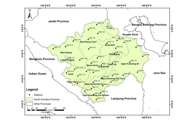
The air quality monitoring system is the most prominent tool for monitoring air pollution levels, especially in areas where forest fires often occur. The South Sumatra Province of Indonesia is one of the greatest contributors to haze events in Indonesia due to peatlands fires. It does not sufficiently possess a ground monitoring system to cover rural areas, and thus, delayed actions can result in severe air pollution within this region. Therefore, the aim of this current study is to analyze the distribution and classification of PM2.5 observed from 2019 to 2021 within the South Sumatra Province, Indonesia. The acquisition of PM2.5 data was from the Merra-2 Satellite with a spatial resolution of 0.5˚ × 0.625˚ and an hourly interval. The hierarchical cluster analysis (HCA) was applied in this study for the clustering method. The result of the study revealed that the daily mean of PM2.5 levels varied from 5.9±0.01 to 21.3±0.03 μg/m3. The study area was classified into three classes: high pollution areas (HPA), moderate pollution areas (MPA) and low pollution areas (LPA), based on the HCA method. The average level of PM2.5 observed in HPA was notably higher, at 16.8±0.02 μg/m3, followed by MPA and LPA. Furthermore, this study indicated that the highest level of PM2.5 was found during 2019, with a severe haze event in the study area due to the intensive burning of forests, bush and peatlands. As a whole, the output of this study can be used by authorities for air quality management due to forest fire events in a certain area.
Citation: Muhammad Rendana, Wan Mohd Razi Idris, Sahibin Abdul Rahim. Clustering analysis of PM2.5 concentrations in the South Sumatra Province, Indonesia, using the Merra-2 Satellite Application and Hierarchical Cluster Method[J]. AIMS Environmental Science, 2022, 9(6): 754-770. doi: 10.3934/environsci.2022043
The air quality monitoring system is the most prominent tool for monitoring air pollution levels, especially in areas where forest fires often occur. The South Sumatra Province of Indonesia is one of the greatest contributors to haze events in Indonesia due to peatlands fires. It does not sufficiently possess a ground monitoring system to cover rural areas, and thus, delayed actions can result in severe air pollution within this region. Therefore, the aim of this current study is to analyze the distribution and classification of PM2.5 observed from 2019 to 2021 within the South Sumatra Province, Indonesia. The acquisition of PM2.5 data was from the Merra-2 Satellite with a spatial resolution of 0.5˚ × 0.625˚ and an hourly interval. The hierarchical cluster analysis (HCA) was applied in this study for the clustering method. The result of the study revealed that the daily mean of PM2.5 levels varied from 5.9±0.01 to 21.3±0.03 μg/m3. The study area was classified into three classes: high pollution areas (HPA), moderate pollution areas (MPA) and low pollution areas (LPA), based on the HCA method. The average level of PM2.5 observed in HPA was notably higher, at 16.8±0.02 μg/m3, followed by MPA and LPA. Furthermore, this study indicated that the highest level of PM2.5 was found during 2019, with a severe haze event in the study area due to the intensive burning of forests, bush and peatlands. As a whole, the output of this study can be used by authorities for air quality management due to forest fire events in a certain area.

| [1] |
Xue Y, Chu J, Li Y, et al. (2020) The influence of air pollution on respiratory microbiome: A link to respiratory disease. Toxicology Letters 334: 14–20. https://doi.org/10.1016/j.toxlet.2020.09.007 doi: 10.1016/j.toxlet.2020.09.007

|
| [2] |
Copat C, Cristaldi A, Fiore M, et al. (2020) The role of air pollution (PM and NO2) in COVID-19 spread and lethality: a systematic review. Environmental research 191: 110129. https://doi.org/10.1016/j.envres.2020.110129 doi: 10.1016/j.envres.2020.110129
|
| [3] | Harishkumar KS, Yogesh KM, Gad I (2020) Forecasting air pollution particulate matter (PM2. 5) using machine learning regression models. Procedia Computer Science 171, 2057–2066. https://doi.org/10.1016/j.procs.2020.04.221 |
| [4] |
Polezer G, Tadano YS, Siqueira HV, et al. (2018) Assessing the impact of PM2. 5 on respiratory disease using artificial neural networks. Environmental pollution 235: 394–403. https://doi.org/10.1016/j.envpol.2017.12.111 doi: 10.1016/j.envpol.2017.12.111
|
| [5] |
Sun X, Zhao T, Liu D, et al. (2020) Quantifying the influences of PM2. 5 and relative humidity on change of atmospheric visibility over recent winters in an urban area of East China. Atmosphere 11: 461. https://doi.org/10.3390/atmos11050461 doi: 10.3390/atmos11050461
|
| [6] |
Yang HH, Arafath SM, Lee KT, et al. (2018) Chemical characteristics of filterable and condensable PM2. 5 emissions from industrial boilers with five different fuels. Fuel 232: 415–422. https://doi.org/10.1016/j.fuel.2018.05.080 doi: 10.1016/j.fuel.2018.05.080
|
| [7] | Hao Y, Gao C, Deng S, et al. (2019) Chemical characterisation of PM2. 5 emitted from motor vehicles powered by diesel, gasoline, natural gas and methanol fuel. Science of the total Environment 674,128–139. https://doi.org/10.1016/j.scitotenv.2019.03.410 |
| [8] |
Xu H, Ta W, Yang L, et al. (2020) Characterizations of PM2. 5-bound organic compounds and associated potential cancer risks on cooking emissions from dominated types of commercial restaurants in northwestern China. Chemosphere 261: 127758. https://doi.org/10.1016/j.chemosphere.2020.127758 doi: 10.1016/j.chemosphere.2020.127758
|
| [9] |
Goudarzi G, Shirmardi M, Naimabadi A, et al. (2019) Chemical and organic characteristics of PM2. 5 particles and their in-vitro cytotoxic effects on lung cells: The Middle East dust storms in Ahvaz, Iran. Science of The Total Environment 655: 434–445. https://doi.org/10.1016/j.scitotenv.2018.11.153 doi: 10.1016/j.scitotenv.2018.11.153
|
| [10] | Fujii Y, Tohno S, Kurita H, et al. (2021) Characteristics of organic components in PM2. 5 emitted from peatland fires on Sumatra in 2015: Significance of humic-like substances. Atmospheric Environment: X 11, 100116. https://doi.org/10.1016/j.aeaoa.2021.100116 |
| [11] |
Song Z, Fu D, Zhang X, et al. (2018) Diurnal and seasonal variability of PM2. 5 and AOD in North China plain: Comparison of MERRA-2 products and ground measurements. Atmospheric Environment 191: 70–78. https://doi.org/10.1016/j.atmosenv.2018.08.012 doi: 10.1016/j.atmosenv.2018.08.012
|
| [12] |
He L, Lin A, Chen X, et al. (2019) Assessment of MERRA-2 surface PM2. 5 over the Yangtze River Basin: Ground-based verification, spatiotemporal distribution and meteorological dependence. Remote Sensing 11: 460. https://doi.org/10.3390/rs11040460 doi: 10.3390/rs11040460
|
| [13] |
Gueymard CA, Yang D (2020) Worldwide validation of CAMS and MERRA-2 reanalysis aerosol optical depth products using 15 years of AERONET observations. Atmospheric Environment 225: 117216. https://doi.org/10.1016/j.atmosenv.2019.117216 doi: 10.1016/j.atmosenv.2019.117216
|
| [14] |
Franceschi F, Cobo M, Figueredo M (2018) Discovering relationships and forecasting PM10 and PM2. 5 concentrations in Bogotá, Colombia, using artificial neural networks, principal component analysis, and k-means clustering. Atmospheric Pollution Research 9: 912–922. https://doi.org/10.1016/j.apr.2018.02.006 doi: 10.1016/j.apr.2018.02.006
|
| [15] |
Govender P, Sivakumar V (2020) Application of k-means and hierarchical clustering techniques for analysis of air pollution: A review (1980–2019). Atmospheric Pollution Research 11: 40-56. https://doi.org/10.1016/j.apr.2019.09.009 doi: 10.1016/j.apr.2019.09.009
|
| [16] | Gö nenç gil B (2020) Evaluate Turkey's climate classification by clustering analysis method. In Smart geography (pp. 41–53). Springer, Cham. https://doi.org/10.1007/978-3-030-28191-5_4 |
| [17] |
Mahmud S, Sumana FM, Mohsin M, et al. (2021) Redefining homogeneous climate regions in Bangladesh using multivariate clustering approaches. Natural Hazards 1: 1–22. https://doi.org/10.21203/rs.3.rs-633865/v1 doi: 10.21203/rs.3.rs-633865/v1
|
| [18] |
Granato D, Santos JS, Escher GB, et al. (2018) Use of principal component analysis (PCA) and hierarchical cluster analysis (HCA) for multivariate association between bioactive compounds and functional properties in foods: A critical perspective. Trends in Food Science & Technology 72: 83–90. https://doi.org/10.1016/j.tifs.2017.12.006 doi: 10.1016/j.tifs.2017.12.006
|
| [19] | Charikar M, Chatziafratis V, Niazadeh R, et al. (2019) Hierarchical clustering for euclidean data. In The 22nd International Conference on Artificial Intelligence and Statistics (pp. 2721–2730). PMLR. |
| [20] |
Bu J, Liu W, Pan Z, et al. (2020) Comparative study of hydrochemical classification based on different hierarchical cluster analysis methods. International journal of environmental research and public health 17: 9515. https://doi.org/10.3390/ijerph17249515 doi: 10.3390/ijerph17249515
|
| [21] |
Ciaramella A, Nardone D, Staiano A (2020) Data integration by fuzzy similarity-based hierarchical clustering. BMC bioinformatics 21: 1–15. https://doi.org/10.1186/s12859-020-03567-6 doi: 10.1186/s12859-020-03567-6
|
| [22] |
Lubis AR, Lubis M (2020) Optimization of distance formula in K-Nearest Neighbor method. Bulletin of Electrical Engineering and Informatics 9: 326–338. https://doi.org/10.11591/eei.v9i1.1464 doi: 10.11591/eei.v9i1.1464
|
| [23] |
Schober P, Boer C, Schwarte LA (2018) Correlation coefficients: appropriate use and interpretation. Anesthesia & Analgesia 126: 1763–1768. https://doi.org/10.1213/ANE.0000000000002864 doi: 10.1213/ANE.0000000000002864
|
| [24] |
Xu Q, Wang S, Jiang J, et al. (2019) Nitrate dominates the chemical composition of PM2. 5 during haze event in Beijing, China. Science of the Total Environment 689: 1293–1303. https://doi.org/10.1016/j.scitotenv.2019.06.294 doi: 10.1016/j.scitotenv.2019.06.294
|
| [25] |
Yabueng N, Wiriya W, Chantara S (2020) Influence of zero-burning policy and climate phenomena on ambient PM2. 5 patterns and PAHs inhalation cancer risk during episodes of smoke haze in Northern Thailand. Atmospheric Environment 232: 117485. https://doi.org/10.1016/j.atmosenv.2020.117485 doi: 10.1016/j.atmosenv.2020.117485
|
| [26] |
Ly BT, Matsumi Y, Nakayama T, et al. (2018) Characterizing PM2. 5 in Hanoi with new high temporal resolution sensor. Aerosol and air quality research 18: 2487–2497. https://doi.org/10.4209/aaqr.2017.10.0435 doi: 10.4209/aaqr.2017.10.0435
|
| [27] |
Hassan H, Latif MT, Juneng L, et al. (2021) Chemical characterization and sources identification of PM2. 5 in a tropical urban city during non-hazy conditions. Urban Climate 39: 100953. https://doi.org/10.1016/j.uclim.2021.100953 doi: 10.1016/j.uclim.2021.100953
|
| [28] |
Lung SCC, Thi Hien T, Cambaliza MOL, et al. (2022) Research Priorities of Applying Low-Cost PM2. 5 Sensors in Southeast Asian Countries. International Journal of Environmental Research and Public Health 19: 1522. https://doi.org/10.3390/ijerph19031522 doi: 10.3390/ijerph19031522
|
| [29] | Tarigan ML, Nugroho D, Firman B, et al. (2015) Pemutakhiran Peta Rawan Kebakaran Hutan dan Lahan di Provinsi Sumatera Selatan. Sumatera Selatan: Dinas Kehutan Provinsi Sumatera Selatan. |
| [30] |
Warsono W, Antonio Y, Yuwono S (2021) Modeling generalized statistical distributions of PM2. 5 concentrations during the COVID-19 pandemic in Jakarta, Indonesia. Decision Science Letters 10: 393–400. https://doi.org/10.5267/j.dsl.2021.1.005 doi: 10.5267/j.dsl.2021.1.005
|
| [31] |
Wu J, Zheng H, Zhe F, et al. (2018) Study on the relationship between urbanization and fine particulate matter (PM2. 5) concentration and its implication in China. Journal of cleaner production 182: 872–882. https://doi.org/10.1016/j.jclepro.2018.02.060 doi: 10.1016/j.jclepro.2018.02.060
|
| [32] |
Zhou Z, Tan Q, Liu H, et al. (2019) Emission characteristics and high-resolution spatial and temporal distribution of pollutants from motor vehicles in Chengdu, China. Atmospheric Pollution Research 10: 749-758. https://doi.org/10.1016/j.apr.2018.12.002 doi: 10.1016/j.apr.2018.12.002
|
| [33] |
Kalisa E, Fadlallah S, Amani M, et al. (2018) Temperature and air pollution relationship during heatwaves in Birmingham, UK. Sustainable cities and society 43: 111–120. https://doi.org/10.1016/j.scs.2018.08.033 doi: 10.1016/j.scs.2018.08.033
|
| [34] |
Taufik M, Widyastuti MT, Sulaiman A, et al. (2022) An improved drought-fire assessment for managing fire risks in tropical peatlands. Agricultural and Forest Meteorology 312: 108738. https://doi.org/10.1016/j.agrformet.2021.108738 doi: 10.1016/j.agrformet.2021.108738
|
| [35] |
Rondhi M, Pratiwi PA, Handini VT, et al. (2018) Agricultural land conversion, land economic value, and sustainable agriculture: A case study in East Java, Indonesia. Land 7: 148. https://doi.org/10.3390/land7040148 doi: 10.3390/land7040148
|
| [36] |
Zhou Y, Li X, Liu Y (2020) Land use change and driving factors in rural China during the period 1995-2015. Land Use Policy 99: 105048. https://doi.org/10.1016/j.landusepol.2020.105048 doi: 10.1016/j.landusepol.2020.105048
|
| [37] |
Li J, Bai Y, Alatalo JM. (2020). Impacts of rural tourism-driven land use change on ecosystems services provision in Erhai Lake Basin, China. Ecosystem Services 42: 101081. https://doi.org/10.1016/j.ecoser.2020.101081 doi: 10.1016/j.ecoser.2020.101081
|
| [38] |
Campbell-Lendrum D, Prüss-Ustün A (2019) Climate change, air pollution and noncommunicable diseases. Bulletin of the World Health Organization, 97: 160. https://doi.org/10.2471/BLT.18.224295 doi: 10.2471/BLT.18.224295
|
| [39] |
Xie J, Liao Z, Fang X, et al. (2019) The characteristics of hourly wind field and its impacts on air quality in the Pearl River Delta region during 2013–2017. Atmospheric Research 227: 112–124. https://doi.org/10.1016/j.atmosres.2019.04.023 doi: 10.1016/j.atmosres.2019.04.023
|
| [40] | Sari NA, Putra RA (2020) Analisis Statistik Deskriptif Titik Panas di Wilayah Sumatera Selatan. In Prosiding Seminar Nasional Sains dan Teknologi Terapan (Vol. 3, No. 1, pp. 51-57). |
| [41] |
Singh RP, Chauhan A (2020) Impact of lockdown on air quality in India during COVID-19 pandemic. Air Quality, Atmosphere & Health 13: 921–928. https://doi.org/10.1007/s11869-020-00863-1 doi: 10.1007/s11869-020-00863-1
|
| [42] |
Dias D, Tchepel O (2018) Spatial and temporal dynamics in air pollution exposure assessment. International journal of environmental research and public health 15: 558. https://doi.org/10.3390/ijerph15030558 doi: 10.3390/ijerph15030558
|
| [43] | Suroto A, Shith S, Yusof NM, et al. (2020) Impact of high particulate event on the indoor and outdoor fine particulate matter concentrations during the Southwest monsoon season. In IOP Conference Series: Materials Science and Engineering (Vol. 920, No. 1, p. 012007). IOP Publishing. https://doi.org/10.1088/1757-899X/920/1/012007 |
| [44] |
Rendana M (2021) Air pollutant levels during the large-scale social restriction period and its association with case fatality rate of COVID-19. Aerosol and Air Quality Research 21: 200630. https://doi.org/10.4209/aaqr.200630 doi: 10.4209/aaqr.200630
|
| [45] |
Rendana M, Idris WMR, Rahim SA (2021) Spatial distribution of COVID-19 cases, epidemic spread rate, spatial pattern, and its correlation with meteorological factors during the first to the second waves. Journal of infection and public health, 14: 1340–1348. https://doi.org/10.1016/j.jiph.2021.07.010 doi: 10.1016/j.jiph.2021.07.010
|
| [46] |
Rendana M, Idris WMR, Rahim SA, et al. (2019) Effects of Organic Amendment on Soil Organic Carbon in Treated Soft Clay in Paddy Cultivation Area. Sains Malaysiana 48: 61–68. https://doi.org/10.17576/jsm-2019-4801-07 doi: 10.17576/jsm-2019-4801-07
|
| [47] | Rendana, M, Idris, WMR (2021) New COVID-19 variant (B. 1.1. 7): forecasting the occasion of virus and the related meteorological factors. Journal of infection and public health, 14: 1320–1327. https://doi.org/10.1016/j.jiph.2021.05.019 |


Figures(9) / Tables(2)

Muhammad Rendana, Wan Mohd Razi Idris, Sahibin Abdul Rahim. Clustering analysis of PM2.5 concentrations in the South Sumatra Province, Indonesia, using the Merra-2 Satellite Application and Hierarchical Cluster Method[J]. AIMS Environmental Science, 2022, 9(6): 754-770. doi: 10.3934/environsci.2022043


 DownLoad: