
Citation: Joje Mar P. Sanchez, Marchee T. Picardal, Marnan T. Libres, Hedeliza A. Pineda, Ma. Lourdes B. Paloma, Judelynn M. Librinca, Reginald Raymund A. Caturza, Sherry P. Ramayla, Ruby L. Armada, Jay P. Picardal. Characterization of a river at risk: the case of Sapangdaku River in Toledo City, Cebu, Philippines[J]. AIMS Environmental Science, 2020, 7(6): 559-574. doi: 10.3934/environsci.2020035
[1] | Sumaiya Noor, Salman A. AlQahtani, Salman Khan . Chronic liver disease detection using ranking and projection-based feature optimization with deep learning. AIMS Bioengineering, 2025, 12(1): 50-68. doi: 10.3934/bioeng.2025003 |
[2] | Wallace Camacho Carlos, Alessandro Copetti, Luciano Bertini, Leonard Barreto Moreira, Otávio de Souza Martins Gomes . Human activity recognition: an approach 2D CNN-LSTM to sequential image representation and processing of inertial sensor data. AIMS Bioengineering, 2024, 11(4): 527-560. doi: 10.3934/bioeng.2024024 |
[3] | Kayode Oshinubi, Augustina Amakor, Olumuyiwa James Peter, Mustapha Rachdi, Jacques Demongeot . Approach to COVID-19 time series data using deep learning and spectral analysis methods. AIMS Bioengineering, 2022, 9(1): 1-21. doi: 10.3934/bioeng.2022001 |
[4] | Abdulmajeed Alsufyani . Performance comparison of deep learning models for MRI-based brain tumor detection. AIMS Bioengineering, 2025, 12(1): 1-21. doi: 10.3934/bioeng.2025001 |
[5] | Marianthi Logotheti, Eleftherios Pilalis, Nikolaos Venizelos, Fragiskos Kolisis, Aristotelis Chatziioannou . Development and validation of a skin fibroblast biomarker profile for schizophrenic patients. AIMS Bioengineering, 2016, 3(4): 552-565. doi: 10.3934/bioeng.2016.4.552 |
[6] | Shital Hajare, Rajendra Rewatkar, K.T.V. Reddy . Design of an iterative method for enhanced early prediction of acute coronary syndrome using XAI analysis. AIMS Bioengineering, 2024, 11(3): 301-322. doi: 10.3934/bioeng.2024016 |
[7] | Md. Mehedi Hassan, Rezuana Haque, Sheikh Mohammed Shariful Islam, Hossam Meshref, Roobaea Alroobaea, Mehedi Masud, Anupam Kumar Bairagi . NeuroWave-Net: Enhancing epileptic seizure detection from EEG brain signals via advanced convolutional and long short-term memory networks. AIMS Bioengineering, 2024, 11(1): 85-109. doi: 10.3934/bioeng.2024006 |
[8] | Abhimanu Singh, Smita Jain . Enhanced brain tumor detection from brain MRI images using convolutional neural networks. AIMS Bioengineering, 2025, 12(2): 215-224. doi: 10.3934/bioeng.2025010 |
[9] | Lamia Fatiha KAZI TANI, Mohammed Yassine KAZI TANI, Benamar KADRI . Gas-Net: A deep neural network for gastric tumor semantic segmentation. AIMS Bioengineering, 2022, 9(3): 266-282. doi: 10.3934/bioeng.2022018 |
[10] | Vincent Brondani . In vitro analysis of site specific nuclease selectivity by NGS. AIMS Bioengineering, 2021, 8(4): 235-242. doi: 10.3934/bioeng.2021020 |
N6,2′-O-dimethyladenosine (m6Am) is a significant RNA modification that plays a vital role in regulating various cellular processes, including gene expression, RNA stability, and the general integrity of RNA metabolism. This modification occurs at the five untranslated regions (UTRs) of messenger RNA (mRNA), influencing key RNA functions such as capping, translation initiation, and RNA decay [1]. m6Am has been shown to affect the interaction of RNA molecules with RNA-binding proteins, modulating critical processes like RNA splicing, transport, and stability. These modifications help regulate gene expression in response to cellular conditions and environmental cues, making them essential for maintaining cellular homeostasis. The dynamic and reversible nature of m6Am modifications in RNA is crucial for regulating mRNA's fate and ensuring the translation machinery's proper functioning [2]. The m6Am modification has gained attention due to its potential implications in disease pathogenesis and cellular dysfunction. The m6Am is linked to various biological processes, such as cell growth, differentiation, stress responses, and RNA surveillance mechanisms. The m6Am role in regulating mRNA stability suggests that it could regulate gene expression in response to stress or environmental changes, making it an essential factor in cellular adaptation and survival [3],[4]. Similarly, alterations in m6Am modification patterns have been associated with several diseases, including cancer, neurological disorders, and metabolic conditions, highlighting its significance in both health and disease. Its importance and accurate identification of m6Am sites within RNA sequences is essential for advancing the understanding of gene regulation and the molecular mechanisms that govern disease progression [5]. The ability to detect m6Am modifications opens new avenues for therapeutic interventions, enabling the development of targeted strategies for diseases that involve aberrant RNA modifications. As a result, computational methods that allow efficient and precise detection of m6Am sites are critical for advancing research in RNA biology and molecular medicine.
Advancements in computational biology have led to several learning tools for predicting RNA modifications, particularly m6Am. For example, Song et al. [6] introduced MultiRM, an attention-based multi-label neural network capable of predicting 12 RNA modifications simultaneously. Using an attention mechanism, MultiRM identifies modification sites and interprets key sequence contexts, revealing strong associations between different RNA modifications. The model achieves 71.13% accuracy with an MCC of 0.427 and an AUC of 0.805 on sequence-based RNA modification mechanisms. Jiang et al. [7] proposed m6AmPred using the eXtreme gradient boosting with dart (XGBDart) algorithm and EIIP-PseEIIP encoding for feature representation. m6AmPred achieved 73.10% accuracy with an MCC of 0.462 and an AUC of 0.820 on cross-validation. Similarly, Luo et al. [8] developed another model named DLm6Am, i.e., an ensemble deep-learning framework combining one-hot encoding, nucleotide chemical property (NCP), and nucleotide density (ND) for feature extraction. DLm6Am integrates CNN, BiLSTM, and multi-head attention modules, outperforming tools like m6AmPred and MultiRM with 79.55% accuracy, 81.71% sensitivity, 77.40% specificity, MCC of 0.591, and AUC of 0.863 on independent testing data. Recently, Jia et al. [9] proposed EMDL_m6Am, a stacking ensemble model employing one-hot encoding and integrating DenseNet, inflated convolutional network (DCNN), and deep multiscale residual network (MSRN) for feature extraction. EMDL_m6Am achieved 80.98% accuracy, 82.25% sensitivity, 79.72% specificity, MCC of 0.619, and AUC of 0.823 on training data, with independent testing (80.98% accuracy, AUC of 0.8211). Despite advancements, existing methods struggle with limited encoding schemes, inefficient feature selection, and reliance on single deep learning frameworks, leading to suboptimal performance and high computational costs. The lack of explainability in current models significantly hinders the interpretation and improvement of accuracy, robustness, and interpretability in m6Am site prediction techniques.
Based on the aforementioned considerations, in this study, we propose Deep-m6Am, a novel deep learning (DL) model designed to accurately identify m6Am sites in RNA sequences. The model integrates multiple feature extraction techniques, including pseudo single nucleotide composition (PseSNC), pseudo dinucleotide composition (PseDNC), and pseudo trinucleotide composition (PseTNC), to capture complex sequence patterns essential for precise prediction. A SHAP (SHapley Additive exPlanations)-based feature selection mechanism is incorporated to enhance computational efficiency and eliminate irrelevant or redundant features, ensuring that only the most informative features contribute to the model's predictions. The Deep-m6Am framework addresses the limitations of single-model approaches by leveraging a multilayer deep neural network (DNN) classifier, improving robustness and generalizability. The model's performance was rigorously evaluated using 5-fold cross-validation and independent testing. The Deep-m6Am demonstrates state-of-the-art results across multiple evaluation metrics, including accuracy, sensitivity, specificity, AUC, and MCC, outperforming existing models and traditional ML algorithms. Integrating cutting-edge feature extraction, selection, and deep learning methodologies, Deep-m6Am provides a powerful and interpretable tool for predicting RNA modifications. This advancement significantly contributes to RNA biology by offering more profound insights into RNA modifications and their roles in disease mechanisms, opening promising avenues for further research into RNA modification patterns. Therefore, Deep-m6Am is a robust computational framework for addressing key challenges in RNA modification analysis, as illustrated in Figure 1.
The rest of the paper is organized as follows: Section 2 presents material and methods, Section 3 illustrates performance metrics and evaluation, Section 4 provides experimental results and analysis, and the work is concluded in Section 5.
A valid and reliable benchmark dataset is essential for designing a powerful and robust computational model. In this study, we utilized the same benchmark datasets employed by Jia et al. [9]. These sites were regarded as highly confident, providing a solid foundation for accurate and reliable model development. Initially, sample sequences were extracted for the training dataset, as depicted in Eq. 1.
Where T1 represents the total RNA sequences,
Where T2 represents the total RNA sequences,
Dataset | Number of samples | Positive samples | Negative samples |
Cross validation | 3548 | 1774 | 1774 |
Training dataset | 2838 | 1419 | 1419 |
Independent dataset | 710 | 355 | 355 |
Several techniques have been developed to convert DNA, protein, and RNA sequences into discrete mathematical models, maintaining the nucleotides' outstanding features and structural integrity. These methods ensure that the biological sequences are accurately described in numerical formats, enabling computational analysis without losing critical sequence-specific information. Accordingly, several bioinformatics approaches have been developed that can transform RNA sequences into various statistical equations with the preservation of the uniqueness and inherent patterns of the measures [10]–[13]. Following the second rule of Chou's 5-step guidelines, several feature extraction techniques have been implemented in this paper to improve the representation of RNA sequences. These techniques include pseudo K-tuple nucleotide composition (PseKNC), comprising methods like PseSNC (Ƙ = 1), PseDNC (Ƙ = 2), and PseTNC (Ƙ = 3). Feature extraction methods are explained in detail in the next section. The PseKNC approach represents RNA sequences as functional vectors by encoding their composition and sequence patterns. This method suppresses detailed order data, focusing on capturing essential features that suggest similarities between RNA samples. By transforming the sequences into structured mathematical representations, PseKNC facilitates efficient computational analysis while preserving key biological characteristics of the RNA [14]. Let us consider an RNA sequence R with N number of nucleotides, represented in Eq. 3.
Where N represents the number of nucleotides in a RNA sequence (i.e. the length of a RNA sequence) and
The Eq. 3, can be expressed in the general form of the PseKNC as
In RNA sequence representation, T is the transposed vector representing a mathematical transformation, z represents a numeric value typically corresponding to an output or dependent variable in the analysis, and ϕy represents the actual value of the RNA sequence's feature vector and can be computed using Eq. 5.
Where θj represent the jth tier correlation factor or jth rank correlation factor that reflects the sequence order correlation in most contiguous K-tuple nucleotides. λ represents the total number correlation rank and w represents the weight. This paper uses the PseKNC technique to convert the provided sequences into discrete feature vectors while maintaining the sequence order data. By designating different values to K (i.e., K = 1, 2, 3) in Eq. 4, three distinct modes of PseKNC were obtained, i.e., PseSNC (K = 1), PseDNC (K = 2), and PseTNC (K = 3), defined as follows:
This study used three distinct feature extraction methods to encode RNA sequences into discrete feature vectors, as summarized in Table 2. These features include PseSNC, PseDNC, and PseTNC, which integrate pseudo, composition, and transitional probability features to improve the differentiation and interpretation of nucleotide sequences [17]–[19]. All individual features were incorporated to construct a comprehensive hybrid feature vector by capturing diverse sequence-derived attributes. Machine learning models leveraging hybrid features benefit from combining multiple extraction techniques, enhancing predictive performance by effectively capturing complex data patterns. This approach remains a widely adopted strategy in bioinformatics and genomics for improving model interpretability and accuracy.
Feature extraction methods | Features |
Pseudo single nucleotide composition (PseSNC) | 4 |
pseudo dinucleotide composition (PseDNC) | 16 |
Pseudo trinucleotide composition (PseTNC) | 64 |
Hybrid features | 84 |
Feature selection is critical in developing models to improve overall performance and computational efficiency. Feature selection involves identifying and retaining the most informative features while eliminating irrelevant or redundant ones, which can introduce noise and reduce prediction accuracy. This study employs SHAP (SHapley Additive exPlanations) as a robust feature selection technique. SHAP leverages cooperative game theory to quantify the contribution of each feature to the model's predictions, ensuring that only the most significant features are retained [20]. This approach reduces the dataset's dimensionality and enhances the model's interpretability by providing insights into the importance of individual features. By integrating SHAP into the Deep-m6Am framework, the model achieves optimized computational efficiency and improved generalization, enabling more accurate and reliable identification of m6Am sites in RNA sequences. This feature selection strategy is pivotal in addressing the challenges of high-dimensional data and ensuring the model's robustness and scalability. This approach enhances model interpretability and supports robust data analysis; it can be expressed as in Eq. 11.
Where φi represents the SHAP value for the feature i, N is the set of all features, and S is a subset of features excluding i. Then, f(S) is the model's prediction given features in S, and
The network topology of a deep neural network, an algorithm based on machine learning or artificial intelligence inspired by the human brain, includes input and output layers and multiple hidden layers. The mechanism of neuron transmission and activation function in DNN is shown in Figure 2. Unlike traditional processing techniques, DNNs can self-learn and automatically acquire pertinent features from unstructured or raw data. Domains in which DNN has been successfully implemented include speech recognition, NLP (Natural Language Processing) and bioengineering, and imaging [21].
The proposed architecture utilizes fully connected layers to locate m6Am sites in RNA sequences. The input layer comprises 42 nodes linked to a first hidden layer of 32 nodes through weighted connections. A second hidden layer with 16 nodes processes outputs from the first layer, followed by a third and last layer with 8 nodes. Each layer employs the rectified linear unit (ReLU) activation function, enabling the model to detect nonlinear relationships and complex patterns [22]. The output layer uses the sigmoid activation function for normalized binary classification, distinguishing m6Am and non-m6Am sites in RNA sequences.
The Deep-m6Am performance is rigorously evaluated using key metrics, including accuracy (ACC), sensitivity (SN), specificity (SP), Matthews correlation coefficient (MCC), and area under the curve (AUC) [23]. SN measures the model's ability to accurately identify true m6Am sites, while SP evaluates its capacity to predict negative cases correctly. ACC reflects the overall correctness of predictions, MCC provides a balanced classification performance assessment, and AUC highlights the model's ability to distinguish between positive and negative instances. These metrics comprehensively evaluate the model's predictive power, ensuring its reliability and effectiveness in identifying m6Am sites.
Where T+ symbolizes true positives, F+ symbolizes false positives, T- Symbolizes true negatives, and F- false negatives, respectively.
In this section, we analyze the hyperparameters of the Deep-m6Am model to optimize its performance. The key hyperparameters considered include learning rate (LR), batch size, number of layers, neurons per layer, and dropout rate. A dropout rate of 0.5 and L2 regularization (0.001) is applied to prevent overfitting, while Xavier initialization ensures stable weight distribution. The model is trained using the Adam optimizer with a learning rate of 0.01 and a momentum of 0.9 to accelerate convergence. Training is conducted for 100 epochs, utilizing ReLU activation functions in the hidden layers and Softmax activation in the output layer for effective learning and classification. A grid search technique was employed to assess the proposed model performance under various hyperparameters, exploring different combinations of parameters. Specifically, the analysis focused on the hyperparameters that significantly influence the performance of the DNN model, including the activation function, learning rate, and number of iterations. Table 3 presents the optimal hyperparameters for the Deep-m6Am.
Parameter | Optimal value |
Dropout rate | 0.5 |
Weight initialization function | Xavier |
Seed | 12345L |
Dropout | 0.001 |
Number of hidden layers | 3 |
Optimizer | Adam, SGD |
L2 regularization | 0.001 |
Epochs | 100 |
Learning rate | 0.01 |
Batch size | 16 |
Activation functions | ReLU, Softmax |
Momentum | 0.9 |
In this section, we conduct the performance analysis of the proposed Deep-m6Am model. We conducted experiments to examine the effects of LR. Table 4 presents a detailed comparison of performance metrics across different learning rates and shows how the chosen learning rate significantly impacts the model's effectiveness and reliability.
LR | ACC (%) | SN (%) | SP (%) | MCC |
0.01 | 83.43 | 82.64 | 84.22 | 0.669 |
0.02 | 80.05 | 79.71 | 80.38 | 0.601 |
0.03 | 79.43 | 80.27 | 78.58 | 0.589 |
0.04 | 78.86 | 78.58 | 79.14 | 0.577 |
0.05 | 78.70 | 75.00 | 82.40 | 0.672 |
As shown in Table 4, the Deep-m6Am model achieves optimal performance with a learning rate of 0.01, attaining the highest accuracy (ACC) of 83.43%, sensitivity (SN) of 82.64%, specificity (SP) of 84.22%, and MCC of 0.669. However, as the learning rate increases, the model's performance declines, highlighting that excessively higher learning rates negatively influence overall metrics.
Furthermore, in Figure 3, we analyze the model's fluctuation in performance with different dropout rates, offering valuable guidance for optimizing this hyperparameter. Proper optimization is crucial for balancing generalization and overfitting prevention, ensuring a robust and reliable model. Figure 3 shows that the model achieves optimal performance at a dropout rate of 0.5, with the highest ACC (83.43%) and MCC (66.90%). Performance improves as the dropout rate increases from 0.1 to 0.5, highlighting 0.5 as the most effective rate for balancing generalization and accuracy.
Moreover, we analyze the effect of varying batch sizes on model performance, comparing outcomes across different sizes to identify optimal configurations. Figure 4 illustrates the impact of batch size on model performance, showing a decline as the batch size increases from 16 to 256. The model achieves optimal performance at a batch size of 16, with the highest ACC (83.43%) and MCC (69.90%). As batch size increases, performance gradually decreases, emphasizing the importance of tuning this hyperparameter for optimal results.
Evaluating the robustness of statistical learning models is essential, and this is typically achieved through validation techniques such as jackknife, k-fold cross-validation, and subsampling. Among these methods, k-fold cross-validation is particularly effective for objectively assessing model performance by dividing the dataset into multiple test sets. This approach ensures a thorough evaluation of the model's generalizability and reliability. Table 5 presents a performance comparison of the proposed Deep-m6Am model using various feature extraction techniques, including individual, hybrid, and SHAP-based feature selection methods.
Method | ACC (%) | SN (%) | SP (%) | MCC |
PseSNC | 71.70 | 66.55 | 76.40 | 0.570 |
PseDNC | 77.73 | 76.89 | 78.58 | 0.555 |
PseTNC | 79.43 | 80.27 | 78.58 | 0.589 |
Hybrid features | 80.83 | 80.27 | 81.40 | 0.617 |
Hybrid features after SHAP | 83.43 | 82.64 | 84.22 | 0.669 |
Table 5 highlights the varying predictive performance of individual features, with PseSNC, PseDNC, and PseTNC achieving ACCs of 71.70%, 77.73%, and 79.43%, respectively. The hybrid feature approach significantly improves classification, reaching an ACC of 80.83%. Further enhancement through SHAP-based feature selection optimizes feature importance, achieving the highest ACC (83.43%) and MCC (0.669). These results underscore the effectiveness of hybrid features in capturing complex patterns and the role of SHAP in refining feature selection for improved model performance.
In this section, we provide an analysis of the DNN model in comparison to well-known machine learning algorithms such as K-nearest neighbor (KNN), random forest (RF), decision tree (DT), naive Bayes (NB), and support vector machine (SVM) [16],[24]–[26]. Table 6 illustrates the importance of evaluating model performance across different classifiers. We employed a 5-fold cross-validation scheme to ensure a reliable and unbiased performance assessment.
Classifiers | ACC (%) | SN (%) | SP (%) | MCC |
RF | 68.72 | 66.91 | 70.53 | 0.667 |
DT | 71.80 | 70.22 | 73.38 | 0.706 |
KNN | 77.15 | 75.62 | 78.68 | 0.741 |
NB | 79.99 | 78.35 | 81.63 | 0.712 |
SVM | 82.53 | 81.96 | 83.09 | 0.651 |
Deep-m6Am | 83.43 | 82.64 | 84.22 | 0.669 |
Table 6 shows that Deep-m6Am outperforms other ML algorithms, achieving the highest ACC (83.43%) and MCC (0.669). SVM follows with an ACC of 82.53%, while NB and KNN achieve 79.99% and 77.15%, respectively. DT (71.80%) and RF (68.72%) perform lower. These results highlight Deep-m6Am as the most effective model for m6Am site identification. To analyze further, we evaluate the proposed model performance using the Area Under the ROC Curve (AUC), as shown in Figure 5. Figure 5 show that the proposed model achieved an AUC value of 0.853, indicating excellent performance compared with widely used ML algorithms.
Furthermore, Table 7 evaluates various ML algorithms on an independent dataset to assess generalizability and robustness. From Table 7, the proposed Deep-m6Am model demonstrated superior performance among the ML classifiers, achieving an ACC of 82.86% with an MCC of 0.657%. The SVM classifier had an ACC of 81.64% with an MCC of 0.632. In contrast, KNN achieved an ACC of 75.45%, while NB, DT, and RF performed at 77.29%, 68.88%, and 66.22%, respectively. This analysis identifies Deep-m6Am as the top-performing model, showcasing its superiority in handling dataset complexities and ensuring reliable and accurate m6Am site prediction.
Classifiers | ACC (%) | SN (%) | SP (%) | MCC |
RF | 66.22 | 64.50 | 68.00 | 0.325 |
DT | 68.88 | 67.10 | 70.66 | 0.378 |
KNN | 75.45 | 73.20 | 77.70 | 0.509 |
NB | 77.29 | 75.20 | 79.38 | 0.545 |
SVM | 81.64 | 79.50 | 83.78 | 0.632 |
Deep-m6Am | 82.86 | 83.65 | 82.07 | 0.657 |
In this section, we conduct a detailed comparative analysis of the proposed Deep-m6Am predictor against several state-of-the-art predictors, including MultiRM [6], m6AmPred [7], DLm6Am [8], and EMDL_m6Am [9]. This comparison is shown in Table 8.
Predictor | ACC (%) | SN (%) | SP (%) | MCC |
MultiRM [6] | 71.13 | 78.59 | 63.66 | 0.427 |
m6AmPred [7] | 73.10 | 72.11 | 74.08 | 0.462 |
DLm6Am [8] | 79.55 | 81.71 | 77.40 | 0.591 |
EMDL_m6Am [9] | 80.98 | 82.25 | 79.72 | 0.619 |
Deep-m6Am | 82.86 | 83.65 | 82.07 | 0.657 |
From Table 8, the MultiRM achieved an ACC of 71.13% and MCC of 0.427, while m6AmPred had an ACC of 73.10% and MCC of 0.462. DLm6Am demonstrated an ACC of 79.55% and MCC of 0.591, and EMDL_m6Am obtained an ACC of 80.98% and MCC of 0.619. In comparison, the proposed Deep-m6Am outperformed all these models, achieving the highest ACC of 82.86% and MCC of 0.657. These results highlight the superior predictive accuracy and robustness of Deep-m6Am for m6Am site identification, making it the most effective model among the evaluated predictors.
The biological function of N6,2′-O-dimethyladenosine (m6Am) in RNA sequences underscores its critical role in regulating post-transcriptional processes, RNA stability, and translation. This study introduces the Deep-m6Am model, which employs a hybrid feature extraction approach, incorporating SHAP (SHapley Additive exPlanations) feature selection and DNN classifier to precisely identify m6Am sites within RNA sequences. Through 5-fold cross-validation, compared with popular ML methods, Deep-m6Am demonstrated unique advantages that resulted in more precise m6Am site predictions. Furthermore, the proposed Deep-m6Am model showed superior performance metrics, achieving an average accuracy of 82.86% compared to the existing models. These results underscore the potential of Deep-m6Am as a reliable and efficient tool for advancing RNA modification analysis.
Future research could expand Deep-m6Am to analyze other RNA modifications and integrate multi-omics data for enhanced predictive accuracy. Exploring its role in disease-specific studies could advance precision medicine. Optimizing computational efficiency through transfer learning, hyperparameter optimization, and parallel programming will improve the model's scalability and applicability in RNA biology and medical research [27].
[1] | Gorme JB, Maniquiz MC, Song P, et al. (2010) The water quality of the Pasig River in the City of Manila, Philippines: Current status, management and future recovery. Environ Eng Res 15: 173–179. |
[2] | Catchilar GC (2008) Fundamentals of Environmental Science. Mandaluyong City: National Book Store. |
[3] | Mora C, Tittensor DP, Adl S, et al. (2011) How many species are there on Earth and in the ocean? PLoS Biol 9: e1001127. |
[4] | Shiklomanov L (1993) World freshwater resources. Water in crisis: A guide to the fresh water resources. New York: Oxford University Press, 13–24. |
[5] | Gleick PH (1996) Water resources. Encyclopedia of climate and weather. New York: Oxford University Press, 2: 817–823. |
[6] | Lansing JS, Lansing P, Erazo J (1998) The value of a river. J Pol Ecol 5: 1–22. |
[7] | Jordaan JM (2009) The uses of river water and impacts. Fresh Surface Water 3: 1–10. |
[8] | Environmental Management Bureau (2014) National water quality report 2006–2013. Quezon City: Department of Environment and Natural Resources-EMB. |
[9] | World Bank (2003) Philippines – environment monitor 2003. Available from: http://documents1.worldbank.org/curated/en/144581468776089600/pdf/282970PH0Environment0monitor.pdf |
[10] | Dyer SD, Peng C, McAvoy DC, et al. (2003) The influence of untreated wastewater to aquatic communities in the Balatuin River, the Philippines. Chemosphere 52: 43–53. |
[11] | Environmental Management Bureau (2016) Annual Report for CY 2016. Quezon City: Department of Environment and Natural Resources-EMB. |
[12] | Picardal JP, Bendoy A, Calumba JR, et al. (2012) Impacts of waste disposal practices and water utilization of riverside dwellers on physico-chemical and microbiological properties of Butuanon River, Central Visayas, Philippines. CNU J High Educ Sp.: 78–100. |
[13] | Oquiñena-Paler, MKM, Ancog, R (2014) Copper, lead and zinc concentration in water, sediments and catfish (Clarias macrocephalus gunther) from Butuanon River, Metro Cebu, Philippines. IOSR J Environ Sci Toxicol Food Tech 8: 49–56. |
[14] | Lo JM, Sakamoto H. Heavy metals distribution in the surface sediments from central west coast of Cebu, Philippines. J Sediment Sco Jap 62: 31–41. |
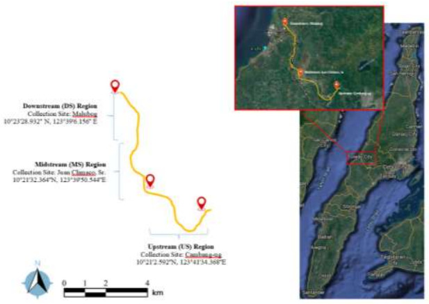
[15] | Paringit, EC, Otadoy, RS (2017) LiDAR surveys and Flood mapping of Sapangdaku River. Quezon City: University of the Philippines Training Center for Applied Geodesy and Photogrammetry. |
[16] | American Public Health Association, American Water Works Association, & Water Environment Association (2005) Standard methods for the examination of water and wastewater (21st Edition). Washington, DC: APHA-AWWA-WEF. |
[17] | Environmental Protection Agency (2012) 5.1 Stream flow. Available from: https://archive.epa.gov/water/archive/web/html/vms51.html |
[18] | Environmental Protection Agency (2012) 5.9 Conductivity. Available from: https://archive.epa.gov/water/archive/web/html/vms59.html |
[19] | Minnesota Pollution Control Agency (2008) Turbidity: description, impact on water quality, sources, measures- A general overview. Available from: https://www.pca.state.mn.us/sites/default/files/wq-iw3-21.pdf |
[20] | National Institute of Water and Atmospheric Research (2016) Streamflow. Available from: https://niwa.co.nz/ |
[21] | Ling TY, Soo CL, Liew JJ, et al. (2017) Application of multivariate statistical analysis in evaluation of surface river water quality of a tropical river. J Chem 2017. |
[22] | Byrne P, Wood PJ, Reid I (2012) The impairment of river systems by metal mine contamination: A review including remediation options. Crit Rev Environ Sci Technol 42: 2017–2077. |
[23] | Haddaway NR, Cooke SJ, Lesser P, et al. (2019) Evidence of the impacts of metal mining and the effectiveness of mining mitigation measures on social–ecological systems in Arctic and boreal regions: a systematic map protocol. Environ Evid 8. |
[24] | Atlas Mining (2013) Safeguarding the natural balance of the environment[Internet] |
[25] | Maglangit FF, Galapate RP, Bensig, EO (2014) Physicochemical-assessment of the water quality of Buhisan River, Cebu, Philippines. Int J Res Environ Sci Tech 4: 83–87 |
[26] | Maglangit FF, Galapate RP, Bensig, EO (2014) Physicochemical-assessment of the water quality of Bulacao River, Cebu, Philippines. J Biodiv Environ Sci 5: 518–525. |
[27] | Kheira R, Boualem R (2015) Impact of quarry sand exploitation on surface water flow quality—case of El Harrach stream channel, Algeria. Desalin Water Treat 57: 21189–21200. |
[28] | Li H, Shi A, Li M, et al. (2013) Effect of pH, temperature, dissolved oxygen, and flow rate of overlying water on heavy metals release from storm sewer sediments. J Chem Article ID 434012. |
[29] | Nyanti L, Soo C, Danial-Nakhaie M, et al. (2018) Effects of water temperature and pH on total suspended solids tolerance of Malaysian native and exotic fish species. AACL Bioflux 11: 565–573. |
[30] | Regional Aquatics Monitoring Program (2018) Water quality indicators: Temperature and dissolved oxygen. Available from: http://www.ramp-alberta.org/river/water+sediment+quality/chemical/temperature+and+dissolved+oxygen.aspx#:~:text=Water%20temperature%20is%20one%20of,decreases%20as%20water%20temperature%20increases. |
[31] | State Water Resources Control Board (2004) The clean water team guidance compendium for watershed monitoring and assessment. Available from: https://www.waterboards.ca.gov/water_issues/programs/swamp/cwt_guidance.html |
[32] | Halliday, SJ, Skeffington, RA, Bowes, MJ, et al. (2008) The water quality of the River Enbourne, UK: Observation from high-frequency in a rural, lowland river system. Water 6: 150–180. |
[33] | Green JA, Pavlish JA, Merritt RG, et al. (2005) Hydraulic impacts of quarries and gravel pits. Legislative Commission on Minnesota Resources. Available from: https://files.dnr.state.mn.us/publications/waters/hdraulic-impacts-of-quarries.pdf |
[34] | Wood MS (2014) Estimating suspended sediment in rivers using acoustic Doppler meters. US Geological Survey Fact Sheet. US Geological Survey |
[35] | Simon TP (1999) Assessing the sustainability and biological integrity of water resources using fish communities. New York: CRC Press |
[36] | Armstrong DS, Parker GW, Richards TA (2004) Evaluation of streamflow requirements for habitat protection by comparison to streamflow characteristics at index streamflow-gaging stations in Southern New England. US Geological Survey |
[37] | Maine Department of Environmental Protection (2016) Dragonfly & damselfly larvae (Odonata). Available from: https://www.maine.gov/dep/water/monitoring/biomonitoring/sampling/bugs/dragonsanddamsels.html |
[38] | Mesner N, Geiger J (2005) Dissolved Oxygen. Utah State University Extension. Available from: https://extension.usu.edu/waterquality/files-ou/whats-in-your-water/do/NR_WQ_2005-16dissolvedoxygen.pdf |
[39] | Vancouver Water Resources Education Center (2020) Water quality: Temperature, pH and dissolved oxygen. Available from: https://www.cityofvancouver.us/sites/default/files/fileattachments/public_works/page/18517/water_quality_tempph_do.pdf |
[40] | Samudro G, Mangkoedihardjo S (2010) Review on BOD, COD and BOD/COD ratio: A triangle zone for toxic, biodegradable and stable levels. Int J Acad Res 2: 235–239 |
[41] | Jordão, CP, Pereira, MG, Matos, AT, et al. (2005) Influence of domestic and industrial waste discharges on water quality at Minas Gerais State, Brazil. J Braz Chem Soc 16: 241–250 |
[42] | Ogunfowokon AO, Okoh EK, Adenuga AA, et al. (2005) An assessment of the impact of point source pollution from a university sewage treatment oxidation pond on a receiving stream- A preliminary study. J App Sci 5: 36–43 |
[43] | Raisbeck MF, Riker SL, Tate CM, et al. (2008) Water Quality for Wyoming Livestock & Wildlife: A Review of the Literature pertaining to Health Effects of Inorganic Contaminants. University of Wyoming Department of Veterinary Sciences |
[44] | Rodrigues ACM, Jesus FT, Fernandes MAF, et al. (2013) Mercury toxicity to freshwater organisms: Extrapolation using species sensitivity distribution. Bull Environ Contam Toxicol, 91: 191–196 |
[45] | Paul S, Mandal A, Bhattacharjee P, et al. (2019) Evaluation of water quality and toxicity after exposure of lead nitrate in fresh water fish, major source of water pollution. Egypt J Aquat Res, 45: 345–351 |
[46] | Woody CA, O'Neal SL (2012) Effects of copper on fish and aquatic resources. The Nature Conservancy. Available from: https://www.conservationgateway.org/ConservationByGeography/NorthAmerica/UnitedStates/alaska/sw/cpa/Documents/W2013ECopperF062012.pdf |
[47] | Oram B (2020) Drinking water and other waters bacterial testing and screening. Water Research Center. Available from: https://water-research.net/index.php/water-testing/bacteria-testing/coliform-bacteria |
[48] | World Health Organization (2003) Guidelines for drinking-water quality. Geneva: WHO |
[49] | Seo M, Lee H, Kim Y (2019) Relationship between coliform bacteria and water quality factors at Weir Stations in the Nakdong River, South Korea. Water 11: 1171 |
[50] | Simeonov V, Stratis JA, Samaraetal C (2003) Assessment of the surface water quality in Northern Greece. Water Res 37: 4119–4124 |
[51] | Bilotta GS, Brazier RE (2008) Understanding the influenceof suspended solids on water quality and aquatic biota. Water Res 42: 2849–2861 |
[52] | Phung D, Huang C, Rutherford S (2015) Temporal and spatial assessment of river surface water quality using multivariate statistical techniques: A study in Can Tho City, a Mekong Deltaarea, Vietnam. Environ Monito Assess 187: 5. |
1. | Sadiah M. A. Aljeddani, Hybrid-DeepLSTM: statistical analysis-based classification of long non-coding RNAs (lncRNAs) in plant genomes using a computational hybrid model enhanced with LSTM layers, 2025, 2731-6688, 10.1007/s43995-025-00128-x | |
2. | Yun Bai, The Role of Education in Building National Soft Power: An Empirical Analysis From a Global Perspective Using Deep Neural Networks, 2025, 13, 2169-3536, 80088, 10.1109/ACCESS.2025.3562589 |
Dataset | Number of samples | Positive samples | Negative samples |
Cross validation | 3548 | 1774 | 1774 |
Training dataset | 2838 | 1419 | 1419 |
Independent dataset | 710 | 355 | 355 |
Feature extraction methods | Features |
Pseudo single nucleotide composition (PseSNC) | 4 |
pseudo dinucleotide composition (PseDNC) | 16 |
Pseudo trinucleotide composition (PseTNC) | 64 |
Hybrid features | 84 |
Parameter | Optimal value |
Dropout rate | 0.5 |
Weight initialization function | Xavier |
Seed | 12345L |
Dropout | 0.001 |
Number of hidden layers | 3 |
Optimizer | Adam, SGD |
L2 regularization | 0.001 |
Epochs | 100 |
Learning rate | 0.01 |
Batch size | 16 |
Activation functions | ReLU, Softmax |
Momentum | 0.9 |
LR | ACC (%) | SN (%) | SP (%) | MCC |
0.01 | 83.43 | 82.64 | 84.22 | 0.669 |
0.02 | 80.05 | 79.71 | 80.38 | 0.601 |
0.03 | 79.43 | 80.27 | 78.58 | 0.589 |
0.04 | 78.86 | 78.58 | 79.14 | 0.577 |
0.05 | 78.70 | 75.00 | 82.40 | 0.672 |
Method | ACC (%) | SN (%) | SP (%) | MCC |
PseSNC | 71.70 | 66.55 | 76.40 | 0.570 |
PseDNC | 77.73 | 76.89 | 78.58 | 0.555 |
PseTNC | 79.43 | 80.27 | 78.58 | 0.589 |
Hybrid features | 80.83 | 80.27 | 81.40 | 0.617 |
Hybrid features after SHAP | 83.43 | 82.64 | 84.22 | 0.669 |
Classifiers | ACC (%) | SN (%) | SP (%) | MCC |
RF | 68.72 | 66.91 | 70.53 | 0.667 |
DT | 71.80 | 70.22 | 73.38 | 0.706 |
KNN | 77.15 | 75.62 | 78.68 | 0.741 |
NB | 79.99 | 78.35 | 81.63 | 0.712 |
SVM | 82.53 | 81.96 | 83.09 | 0.651 |
Deep-m6Am | 83.43 | 82.64 | 84.22 | 0.669 |
Classifiers | ACC (%) | SN (%) | SP (%) | MCC |
RF | 66.22 | 64.50 | 68.00 | 0.325 |
DT | 68.88 | 67.10 | 70.66 | 0.378 |
KNN | 75.45 | 73.20 | 77.70 | 0.509 |
NB | 77.29 | 75.20 | 79.38 | 0.545 |
SVM | 81.64 | 79.50 | 83.78 | 0.632 |
Deep-m6Am | 82.86 | 83.65 | 82.07 | 0.657 |
Predictor | ACC (%) | SN (%) | SP (%) | MCC |
MultiRM [6] | 71.13 | 78.59 | 63.66 | 0.427 |
m6AmPred [7] | 73.10 | 72.11 | 74.08 | 0.462 |
DLm6Am [8] | 79.55 | 81.71 | 77.40 | 0.591 |
EMDL_m6Am [9] | 80.98 | 82.25 | 79.72 | 0.619 |
Deep-m6Am | 82.86 | 83.65 | 82.07 | 0.657 |