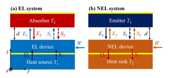
Electroluminescent (EL) and negative electroluminescent (NEL) devices are radiative thermoelectric energy converters that use electric power for refrigeration. For the EL system, we apply a forward bias to the emitter that we want to cool, whereas a reverse bias voltage is applied to the hot absorber for the NEL system. In this work, we derive the thermodynamic limits of the cooling power density and coefficient of performance (COP) of near-field EL and NEL refrigeration systems based on entropy analysis that considers near-field effects. We show numerically that operating the EL and NEL systems in the near-field regime could increase the cooling power density and the COP bounds to a certain extent. As the vacuum gap decrease from 1000 to 10 nm, the near-field effects improve the performance of the NEL system all the time, but the performance of the EL system increases to the optimal value and then decreases. In addition, the increase in temperature difference weakens the performance of both refrigeration systems greatly. Moreover, we also investigate the effects of the absence of sub-bandgap thermal radiation on the performance of the EL and NEL systems. Our work indicates significant opportunities for evaluating the performance of near-field radiative thermoelectric energy converters from the perspective of thermodynamic limits. Meanwhile, these results establish the targets for cooling power density and COP of the near-field EL and NEL systems.
Citation: Bowen Li, Qiang Cheng, Jinlin Song, Kun Zhou, Lu Lu, Zixue Luo. Thermodynamic performance of near-field electroluminescence and negative electroluminescent refrigeration systems[J]. AIMS Energy, 2021, 9(3): 465-482. doi: 10.3934/energy.2021023
| [1] | Hong Lu, Linlin Wang, Mingji Zhang . Studies on invariant measures of fractional stochastic delay Ginzburg-Landau equations on Rn. Mathematical Biosciences and Engineering, 2024, 21(4): 5456-5498. doi: 10.3934/mbe.2024241 |
| [2] | Azmy S. Ackleh, Rainey Lyons, Nicolas Saintier . High resolution finite difference schemes for a size structured coagulation-fragmentation model in the space of radon measures. Mathematical Biosciences and Engineering, 2023, 20(7): 11805-11820. doi: 10.3934/mbe.2023525 |
| [3] | H.T. Banks, S. Dediu, H.K. Nguyen . Sensitivity of dynamical systems to parameters in a convex subset of a topological vector space. Mathematical Biosciences and Engineering, 2007, 4(3): 403-430. doi: 10.3934/mbe.2007.4.403 |
| [4] | D. Criaco, M. Dolfin, L. Restuccia . Approximate smooth solutions of a mathematical model for the activation and clonal expansion of T cells. Mathematical Biosciences and Engineering, 2013, 10(1): 59-73. doi: 10.3934/mbe.2013.10.59 |
| [5] | Azmy S. Ackleh, Rainey Lyons, Nicolas Saintier . Finite difference schemes for a structured population model in the space of measures. Mathematical Biosciences and Engineering, 2020, 17(1): 747-775. doi: 10.3934/mbe.2020039 |
| [6] | Qihua Huang, Hao Wang . A toxin-mediated size-structured population model: Finite difference approximation and well-posedness. Mathematical Biosciences and Engineering, 2016, 13(4): 697-722. doi: 10.3934/mbe.2016015 |
| [7] | Gheorghe Craciun, Matthew D. Johnston, Gábor Szederkényi, Elisa Tonello, János Tóth, Polly Y. Yu . Realizations of kinetic differential equations. Mathematical Biosciences and Engineering, 2020, 17(1): 862-892. doi: 10.3934/mbe.2020046 |
| [8] | Bing Hu, Minbo Xu, Zhizhi Wang, Jiahui Lin, Luyao Zhu, Dingjiang Wang . Existence of solutions of an impulsive integro-differential equation with a general boundary value condition. Mathematical Biosciences and Engineering, 2022, 19(4): 4166-4177. doi: 10.3934/mbe.2022192 |
| [9] | Mario Lefebvre . An optimal control problem without control costs. Mathematical Biosciences and Engineering, 2023, 20(3): 5159-5168. doi: 10.3934/mbe.2023239 |
| [10] | Azmy S. Ackleh, Mark L. Delcambre, Karyn L. Sutton, Don G. Ennis . A structured model for the spread of Mycobacterium marinum: Foundations for a numerical approximation scheme. Mathematical Biosciences and Engineering, 2014, 11(4): 679-721. doi: 10.3934/mbe.2014.11.679 |
Electroluminescent (EL) and negative electroluminescent (NEL) devices are radiative thermoelectric energy converters that use electric power for refrigeration. For the EL system, we apply a forward bias to the emitter that we want to cool, whereas a reverse bias voltage is applied to the hot absorber for the NEL system. In this work, we derive the thermodynamic limits of the cooling power density and coefficient of performance (COP) of near-field EL and NEL refrigeration systems based on entropy analysis that considers near-field effects. We show numerically that operating the EL and NEL systems in the near-field regime could increase the cooling power density and the COP bounds to a certain extent. As the vacuum gap decrease from 1000 to 10 nm, the near-field effects improve the performance of the NEL system all the time, but the performance of the EL system increases to the optimal value and then decreases. In addition, the increase in temperature difference weakens the performance of both refrigeration systems greatly. Moreover, we also investigate the effects of the absence of sub-bandgap thermal radiation on the performance of the EL and NEL systems. Our work indicates significant opportunities for evaluating the performance of near-field radiative thermoelectric energy converters from the perspective of thermodynamic limits. Meanwhile, these results establish the targets for cooling power density and COP of the near-field EL and NEL systems.
Transport type equations arise ubiquitously in the physical, biological and social sciences (e.g., see [1,2,3]). They were, for example, recently used to approximate the dynamics of opinion formation [3] (see also [4] and [5]), to describe flow on networks (see [6,7,8]) and to model the dynamics of structured populations [9]. Because of the natural setting of the space of measures for these equations, as it allows for unifying discrete and continuous dynamics under the same framework, researchers have recently focused their efforts to study well-posedness of such equations on this space [10,11,12]; hence generalizing previous results that treated these equations in the space of integrable functions (e.g, [1]).
The importance of understanding differentiability of solutions of differential equation models with respect to parameters is crucial for many applications including optimal control (e.g., [13,14]), parameter estimation and least-square problems of fitting models to data [15,16], and sensitivity analysis of solutions to model parameters that can be used to obtain information on parameter uncertainty including confidence intervals for estimated model parameters (e.g., [17,18,19]). Such applications require the minimization of a functional that depends on the model solution and hence (numerically) solving for the critical points of the equation that represents the derivative of the solutions with respect to parameter often becomes necessary.
In this paper, we focus on deriving an equation that represents the derivative of a transport equation with respect to the vector field. To this end, consider the following transport equation in the space of bounded, nonnegative Radon measures M+(Rd):
| ∂tμt+∂x(v(x)μt)=0 | (1.1) |
where μt:[0,T]→M+(Rd) and v:Rd→Rd is a given vector field. Equation (1.1) is equipped with the initial condition μ|t=0=μ0. It is well-known that if v∈W1,∞(Rd), this equation has a unique solution in C([0,+∞),M+(Rd)) given by μt=T#tμ0 where Tt is the flow of v (defined in (2.2)) and T#t denotes the push - forward along the map Tt (see Eq (2.5)). Here, the space of measures is endowed with the so-called bounded Lipschitz norm ‖⋅‖BL∗ (see Eq (2.1)).
Here, we focus on the regularity of μt with respect to v, i.e., if v is slightly perturbed, how will μt change? To be more precise, suppose v(x) is replaced with the new vector field vh(x):=v0(x)+hvp(x) where v0 and vp are fixed vector fields and h can vary. The perturbed equation is then
| ∂tμht+∂x(vh(x)μht)=0 | (1.2) |
which has the unique solution μht=(Tht)#μ0 where Tht is the flow of the vector field vh. It is easy to see, using the representation formula for solutions to (1.2) presented in [20] or [21] (Eq 1.3) and estimates similar to the ones used to prove Lemma 3.8 in [22], that the map h↦μh is Lipschitz continuous in C([0,T],M+(Rd)) so that in particular limh→0μh=μ in C([0,T],M+(Rd)) for any T>0 (see also Eq (2.7)).
The next step in understanding the regularity of h↦μht consists in studying the existence of the derivative ∂hμh. This type of questions has been recently addressed in [23] for linear transport equation and for general nonlinear structured population models (including transport equation) in [24]. Briefly, denoting by ρΔht,h:=(μh+Δht−μht)/Δh, a difference quotient, the question is to give a precise mathematical meaning to the limit limΔh→0ρΔht,h. It turns out that this type of problems cannot be answered in the framework of bounded Lipschitz norm (see Example 3.5 in [24]). Indeed it is necessary to move to the bigger space Z defined as the closure of M(Rd) endowed with the dual norm (C1,α(Rd)∗ (see Section 2.3 for a brief introduction). Then, according to Theorem 1.1 in [23], one can prove that there exists ρt,h∈Z such that limΔh→0ρΔht,h=ρt,h (see also Theorem 2.1 below).
In this paper we want to characterize ρ as the unique solution to some equation. In fact, one of the main results in this work (see, Theorem 4.1 below) states that ρ is the unique solution to the equation
| ∂tρt+∂x(v0(x)ρt)=−∂x(vp(x)μt). |
This equation can then be thought of as the sensitivity equation satisfied by the directional derivative of μ under the perturbation v0+hvp. We will also prove an analogous result in the non-linear case when the vector-field v depends on μ (see Theorem 5.1 below).
The proofs of these results require the detailed study of a linear transport equation in Z of the form
| ∂tμt+∂x(v(x)μt)=νt,μ|t=0=μ0. | (1.3) |
While the existence of a solution to (1.3) can be established by extending standard techniques to the current setting on the space Z, the uniqueness issue presents some unexpected difficulties which led to a new notion of solution. With this new concept of solution, we are able to prove in Theorem 3.1 that this equation is well-posed.
The paper is organized as follows. In Section 2 we briefly recall some known facts concerning transport equations in the space of measures and the space Z. We also establish new properties of the space Z. For a smooth flow of the paper we provide the details of long proofs of these new properties in the Appendix. In Section 3, we prove the existence and uniqueness of a solution to linear equation of type (1.3) in Z. This allows to formulate sensitivity equations in the the linear (Section 4) and the nonlinear (Section 5) cases. In Section 6, we discuss possible applications of our results.
We briefly review here the formulation of the transport equation
| ∂tμt+∂x(v(x)μt)=0 |
on the space nonnegative Radon measures M+(Rd). This space is equipped with the bounded Lipschitz norm defined for μ∈M+(Rd) as
| ‖μ‖BL∗=sup‖ψ‖W1,∞(Rd)≤1∫Rdψ(x)dμ(x), | (2.1) |
as the total variation norm is too strong. Here, W1,∞(Rd) is the space of bounded and globally Lipschitz functions.
Let v be a vector field with v∈W1,∞(Rd,Rd). Then, the flow of v denoted by Ttv:Rd→Rd is defined as the solution to the ODE:
| ddt(Ttv)(x)=v((Ttv)(x)),(T0v)(x)=x. | (2.2) |
Notice that (Ttv)(x) is defined for all t∈R. If there is no risk of confusion, we write Tt instead of Ttv. Now, the classical method of characteristics allows to solve the transport equation
| ∂tμt+∂x(v(x)μt)=νt,μt|t=0=μ0, | (2.3) |
where νt∈C([0,T],M+(Rd)). More precisely, the unique measure solution in C([0,T],M(Rd)) to (2.3) is given by propagating the initial condition μ0 along the flow of v, namely
| μt=T#tμ0+∫t0T#t−sνsds, | (2.4) |
where for f:Rd→Rd and measure μ∈M+(Rd), f#μ is the push-forward measure defined as
| f#μ(A)=μ(f−1(A)) for any measurable A⊂Rd. | (2.5) |
We remark here that the definition of the push-forward measure yields the following change of variables formula: for all measurable maps T:Rd→Rd and ϕ:Rd→R,
| ∫Rdϕ(x)d(T#μ)(x)=∫Rdϕ∘T(x)dμ(x). | (2.6) |
For the proof, see [25] for the case ν=0 and Proposition 3.6 in [21]. Let us also note that formula (2.4) is true also in the setting of bounded Radon measures M(Rd): as the equation is linear, one can apply the Hahn-Jordan decomposition (see Section 4.2 in [26]) and solve the equations for the positive and the negative parts of the measure separately.
Now, let v1 and v2 be two bounded and globally Lipschitz vector fields. Let μ(1)t and μ(2)t be the solutions to (2.3) with vector fields v1 and v2, respectively. Then, there is a constant C=C(T,‖v1‖W1,∞,‖v2‖W1,∞,μ0) such that
| ‖μ(1)t−μ(2)t‖BL∗≤C‖v1−v2‖∞,for any t∈[0,T]. | (2.7) |
For the proof, one simply applies the triangle and Gronwall inequalities as in the proof of Lemma 3.8 in [22]. The solution to (2.3) thus depends continuously on v.
The transport equation (2.3) can also be studied in a nonlinear setting where the vector field depends on the measure solution itself. Then, the nonlinear transport equation takes the form
| ∂tμt+∂x(v[μt](x)μt)=0. | (2.8) |
where v:M+(Rd)→W1,∞(Rd,Rd). It is common in application that v depends on μ through some weighted mean of μ of the form
| v[μ](x)=V(x,∫RdKV(x,y)dμ(y)) | (2.9) |
for given maps V:Rd×R→Rd and KV:Rd×Rd→R.
Given α∈(0,1), we consider the space C1,α(Rd) of bounded continuous functions with bounded and α-Hölder derivative endowed with the norm
| ‖u‖C1,α:=‖u‖∞+‖Du‖∞+supx≠y|Du(x)−Du(y)||x−y|α. |
Lemma 2.1. 1. For any u∈C1,α(Rd),
| |u(x+y)−u(y)−∇u(x)y|≤‖∇u‖C0,α|y|1+αfor any x,y∈Rd. | (2.10) |
2. If ϕ∈C1,α(Rd) and T∈C1,α(Rd,Rd) then ϕ∘T∈C1,α(Rd) with norm bounded by a constant depending only on a bound of ‖ϕ‖C1,α and ‖T‖C1,α.
Proof. The first assertion follows from
| u(x+y)−u(y)−∇u(x)y=∫10ddtu(x+ty)−∇u(x)ydt=∫10(∇u(x+ty)−∇u(x))ydt. |
For the second one we only need to estimate |D(ϕ∘T)(x)−D(ϕ∘T)(y)|. We have
| |Dϕ(T(x))DT(x)−Dϕ(T(y))DT(y)|≤|Dϕ(T(x))(DT(x)−DT(y)|+|(Dϕ(T(x))−Dϕ(T(y)))DT(y)|≤‖ϕ‖C1,α‖T‖C1,α|x−y|α+‖ϕ‖C1,α|T(x)−T(y)|α‖T‖C1,α≤C|x−y|α, |
where C=‖ϕ‖C1,α‖T‖C1,α+‖ϕ‖C1,α‖T‖1+αC1,α.
We also recall the following result from Cor. 3.16 in [24] regarding the regularity of the flow Ttv defined in (2.2):
Proposition 2.1. Assume that v∈C1,α(Rd,Rd). Then there exists a constant CT>0 depending only on T and ‖v‖C1,α such that ‖D(Ttv)‖C0,α≤CT for any t∈[0,T]. Moreover it can be checked upon inspection of the proof that CT→1 as T→0.
We consider the space Z defined as the closure of M(Rd) endowed with the dual norm (C1,α(Rd))∗ for some α (see Remark 2.1 on the choice of α). This space was first introduced in [23] where the authors demonstrated that Z has a lot of convenient topological properties. In particular, Z is a separable Banach space with its dual being isometrically isomorphic to C1,α(Rd). Indeed it was proved in [23][Prop. 5.1] that span{δx,x∈Qd} is dense in Z. In particular this implies that any element of Z can be approximated by bounded measures.
Notice that using duality we have for any μ∈Z,
| ‖μ‖Z=sup‖ψ‖C1,α≤1(μ,ψ). |
The main advantage of space Z is its applicability to studying differentiation problems with respect to perturbation of transport equations. More precisely, let us consider Eq (2.3) with νt=0 and vector field v0(x)+hvp(x) where h∈[−M,M] for some M>0, and denote by μht its solution, namely
| ∂tμht+∂x((v0+hvp)μht)=0,μht|t=0=μ0. |
One is then interested in the limit μh+Δht−μhtΔh as Δh→0. The following result was obtained in [23]:
Theorem 2.1. Let v0,vp∈C1+α(Rd,Rd). Then, μh+Δht−μhtΔh converges in C([0,T],Z) as Δh→0.
Remark 2.1. Let Zα=¯M(Rd)(C1,α(Rd))∗. Notice that if 0<α<α′<1 then C1,α′⊂C1,α from which we deduce that Zα⊂Zα′ with continuous injection. Therefore, if incremental quotient μh+Δht−μhtΔh converges in Zα, it also does so in Zα′ for any α′<α. Moreover, since Zα⊂Zα′ continuously, both limits coincide. So there is no ambiguity and we simply write Z instead of Zα.
Such a perturbation problem can be also studied for the nonlinear transport equation (2.8) with a vector-field v0[μ] like (2.9). We perturb v0[μ] considering vh[μ](x) defined as
| vh[μ](x)=v0[μ](x)+hvp[μ](x)=V0(x,∫RdKV0(x,y)dμ(y))+hVp(x,∫RdKVp(x,y)dμ(y)). | (2.11) |
Then, we have the following result:
Theorem 2.2. Let α>12 and vh[μ] be given by (2.11), where V0,Vp∈C1+α(Rd×R,Rd) and KV0,KVp∈C2+α(Rd×Rd,R). Let μht be the unique solution to (2.8) with the vector field vh[μ]. Then, μh+Δht−μhtΔh converges in C([0,T],Z) as Δh→0.
Remark 2.2. The proof of existence and uniqueness of solutions as well as of a differentiability result was actually given only for the case of R+ in [22] and [24] respectively. However, the proof can be easily extended to Rd. Indeed, the main idea is to construct approximating sequence as follows. The interval of time [0,T] is divided into 2k subintervals of the form [lT2k,(l+1)T2k] where l=0,1,...,2k−1. Then, the following approximation is defined recursively: for t∈(lT2k,(l+1)T2k], let μt be the solution to
| ∂tμt+∂x(v[μlT2k](x)μt)=0. |
with initial condition μlT2k. One then uses the formula for the solution of the linear problem (2.4) to conclude the proof. See [22] and [24] for more details.
The following Propositions discuss the distributional derivatives of bounded Radon measures as elements of space Z. For easier flow of this section long proofs are provided in the Appendix.
We can see a Radon measure μ∈M(Rd) as a distribution by (μ,ϕ)=∫ϕdμ, ϕ∈C∞c(Rd). We denote by ∂xϕ:=∇ϕ⋅x the derivative of ϕ in direction x∈Rd. We then define a distribution ∂xμ by duality letting (∂xμ,ϕ)=−(μ,∂xϕ). The next result shows that in fact ∂xμ belongs to Z when μ is bounded.
Proposition 2.2. For any bounded μ∈M(Rd), the distributional derivative ∂xμ of μ in direction x∈Rd belongs to Z.
Proof. Let μ∈M(Rd) be bounded. To prove that the distributional derivative ∂xμ belongs to Z, we need to find a sequence νh∈M(Rd) such that νh→∂xμ as h→0 in Z. Let τh be the translation operator defined by τhϕ(y):=ϕ(y+hx) for any ϕ. Take νh:=(τ#hμ−μ)/h∈M(Rd). Then for any ϕ∈C1,α(Rd) with ‖ϕ‖C1,α(Rd)≤1 we have using (2.10) that
| |(νh,ϕ)−(−∂xμ,ϕ)|=∫Rd|ϕ(y+hx)−ϕ(y)h−∂xϕ(y)|dμ(y)≤|h|α‖μ‖TV |
so that νh→−∂xμ in Z as h→0.
Proposition 2.3. Consider μn,μ∈Mb(Rd) such that μn→μ narrowly (i.e. in duality with bounded and continuous functions Cb(Rd)). Then ∂xμn→∂xμ in Z.
Proof. See Appendix.
,
Proposition 2.4. For a bounded vector field v on Rd and μ∈Mb(Rd) we have
| ‖∂x(vμ)‖Z≤‖μ‖TV‖v‖∞. | (2.12) |
Moreover, consider measures μn,μ∈Mb(Rd) such that μn→μ narrowly and vector fields vn,v∈Cb(Rd,Rd) such that vn→v uniformly. Then ∂x(vnμn)→∂x(vμ) in Z.
Proof. For any ϕ such that ‖ϕ‖C1,α≤1 we have
| |(∂x(vμ),ϕ)|=|(μ,v∂xϕ)|≤‖μ‖TV‖v∂xϕ‖∞≤‖μ‖TV‖v‖∞. |
Then, in view of Proposition 2.3, to verify the second assertion, it is sufficient to prove that vnμn→vμ narrowly. For ϕ∈Cb(Rd), we have
| (vnμn−vμ,ϕ)=(μn,(vn−v)ϕ)+(μn−μ,vϕ) |
where (⋅,⋅) denotes the dual pairing. The first term can be bounded by ‖μn‖TV‖(vn−v)ϕ‖∞≤C‖(vn−v)‖∞→0 while the second tends to 0 since vϕ∈Cb(Rd).
We deduce that
Corollary 2.1. Let [0,T]∋t↦μt∈Mb(Rd) be a narrowly continuous map and v∈Cb(Rd,Rd). Then ∂x(vμt)∈C([0,T],Z).
It will also be useful to define the push-forward of an element of Z. The idea is quite simple. In fact, since this is well-defined on the space of measures, we can extend its definition for elements of Z by means of Cauchy sequences.
Proposition 2.5. Let T∈C1,α(Rd,Rd). Then for any μ∈Z we can define T#μ∈Z by
| T#μ:=limn→∞T#μn |
where {μn}n∈N⊂M(Rd) is any sequence such that μn→μ in Z. Then, for any ϕ∈C1,α(Rd) we have the following analogue of the change of variables formula (2.6):
| (T#μ,ϕ)=(μ,ϕ∘T) |
where ϕ∘T denotes composition of the maps ϕ and T.
Proof. See Appendix.
We conclude this section with the following classical observation. By definition, if μ∈Z, there is a sequence of bounded measures {μn}n∈N such that μn→μ in Z. Now, if μ∈C([0,T],Z), for each t∈[0,T], one can choose an approximating sequence for each μt, t∈[0,T]. However, it is possible to construct an approximating sequence that is continuous in time and so, that approximates the whole curve t↦μt, t∈[0,T]. This is the content of the following lemma.
Lemma 2.2. Let μ∈C([0,T],Z). There is a sequence {μ(n)}n∈N⊂C([0,T],Mb(Rd)) such that μ(n)→μ in C([0,T],Z) as n→∞.
Proof. See Appendix.
Corollary 2.2. Let ν∈C([0,T],Z) and v∈C1,α(Rd). Then the map t→Ttv#νt is continuous from [0,T] to Z.
Proof. See Appendix.
In this section, we study the following transport equation in the space Z:
| ∂tμt+∂x(v(x)μt)=νt,μ|t=0=μ0, | (3.1) |
where v∈C1,α(Rd,Rd), ν∈C([0,T],Z) and μ0∈Z. We begin with a concept of a very weak solution.
Definition 3.1. We say that μ∈C([0,T],Z) is a very weak solution to (3.1) in Z if for any φ∈C([0,T]×Rd) with φ∈C([0,T],C2+α(Rd)) and φt∈C([0,T],C1+α(Rd)) we have:
| (μT,φ(x,T))=(μ0,φ(x,0))+∫T0(μt,φt(.,t)+v⋅∇φ(.,t))dt+∫T0(νt,ϕ(.,t))dt. | (3.2) |
Note that we have to use test functions of regularity at least C2+α in space variable x so that function φt+v(x)⋅∇xφ lies in Z, the domain of the functional μt.
Proposition 3.1. Equation (3.1) has at least one very weak solution in C([0,T],Z) given by
| μt=T#tμ0+∫t0T#t−sνsds | (3.3) |
where the integral is a Bochner integral in Z.
Moreover, if μ0=0 and νt=0, then for any weak solution μt we have
| (μt,η)=0 | (3.4) |
for all η∈C2+α(Rd) and t∈[0,T].
Proof. We first verify that the integral appearing on the right-hand side of (3.3) is a Bochner integral in Z. According to Corollary 2 the map f:s∈[0,t]→T#t−sνs∈Z is continuous. Thus for any z∗∈Z∗, z∗∘f is also continuous. Since Z is separable, we conclude using Pettis theorem that f is measurable. Moreover for any ϕ∈C1,α(Rd), ‖ϕ‖C1,α≤1, we have
| |(f(s),ϕ)|=|(νs,ϕ∘Tt−s)|≤‖νs‖Z‖ϕ∘Tt−s‖C1,α≤CT |
since ν∈C([0,T],Z) and in view of Lemma 2.1 and Proposition 1. It follows that max0≤s≤t‖f(s)‖Z≤CT and thus that f is Bochner-integrable. It is also easily seen that ∫t0T#t−sνsds is continuous in t.
Let μt be defined by (3.3). Clearly μ∈C([0,T],Z). We now verify that μt is a solution in the sense of Definition 1. According to Lemma 2, we we can find sequences {ν(n)}n∈N⊂C([0,T],Mb(Rd)) and {μn0}n∈N⊂Mb(Rd) such that ‖μ(n)0−μ0‖Z→0 and ‖ν(n)t−νt‖Z→0 uniformly in t∈[0,T]. Then the transport equation
| ∂tμt+∂x(v(x)μt)=ν(n)t,μ|t=0=μ(n)0 | (3.5) |
has a unique solution μ(n)∈C([0,T],Mb(Rd)) given by
| μ(n)t=T#tμ(n)0+∫t0T#t−sν(n)sds. | (3.6) |
According to Proposition 2.5, T#tμ(n)0→T#tμ0 in Z and, for any s, T#t−sν(n)s→T#t−sνs in Z. Since ‖T#t−sν(n)s‖Z≤CT we have applying the Dominated Convergence Theorem that ∫t0T#t−sν(n)sds→∫t0T#t−sνsds in Z. Thus for any t∈[0,T], μ(n)t converges in Z to μt given by
| μt:=limn→+∞μ(n)t=T#tμ0+∫t0T#t−sνsds. |
Clearly, μ∈C([0,T],Z). On the other hand, weak formulation for (3.5) is valid for test functions of class C1([0,T]×Rd)∩W1,∞([0,T]×Rd). In particular, taking test functions as in Definition 3.1, we send n→∞ in the weak formulation for (3.5) to deduce that μt is a very weak solution to (3.1).
To prove (3.4), we use the so-called dual problem (cf. Remark 8.1.5 and Proposition 8.1.7 in [27] or Proposition 5.34 in [25]). More precisely, given some function ψ(x,t), let φ be the solution of
| ∂tφ+v(x)⋅∇xφ=ψ,φ(x,T)=0. | (3.7) |
which is explicitly given by φ(x,t)=−∫Ttψ(Ts−t(x),s)ds. We consider ϕ of the form ψ(x,t)=ξ(t)η(x) where ξ∈C∞c([0,T]) and η∈C2,α(Rd). We then use the corresponding solution ϕ of (3.7) as a test function in (3.2) to conclude
| ∫T0ξ(t)(μt,η)dt=0. |
Since the map t↦(μt,η(x)) is continuous for t∈[0,T] and since ξ is arbitrary, we deduce that (μt,η)=0 for any η∈C2,α(Rd) and t∈[0,T].
Unfortunately, condition (3.4) does not imply that μt=0 so that we cannot deduce the uniqueness of a solution to (3.1). The problem here is that C2+α(Rd) is not dense in C1+α(Rd). The following two examples shows the typical problem with approximation of Hölder functions.
Example 3.1. One can easily check that f(x)=√x∈C1/2([0,1]). Suppose there is a sequence {fn}n∈N⊂C1([0,1]) such that ‖fn−f‖C1/2→0. Then
| 0←‖fn−f‖C1/2≥supx∈(0,1]|1−fn(x)−fn(0)√x|≥supx∈(0,1]|fn(x)−fn(0)|√x−1, |
contradicting {fn}n∈N⊂C1([0,1]).
Example 3.2. We construct a nontrivial functional on C1/2([0,1]) which vanishes on C1,1/2([0,1]). In particular, this shows that functionals on C1/2([0,1]) cannot be uniquely characterized by their values on C1,1/2([0,1]). Let X=C1([0,1])⊕lin(√x) be a linear subspace of C1/2([0,1]). On X, we can define a functional φ:X→R with
| φ(f)=limx→0f(x)−f(0)√x. |
Notice that ϕ is continuous since |φ(f)|≤‖f‖C1/2. By the analytic version of Hahn-Banach Theorem (Theorem 1.1 in [28]), we can then extend φ to a continuous functional on C1/2([0,1]). It is easily seen that ϕ(f)=0 for any f∈C1([0,1]) by Taylor's estimate but that φ(√x)=1.
There is also characterization of subset in Cα consisting of functions that can be approximated by smooth functions:
Remark 3.1. Let Ω⊂Rd. Then, f∈Cα(Ω) can be approximated by smooth functions if and only if f is an element of the set
| Fα(Ω)={f∈Cα(Ω):limt→0+sup|x−y|≤t|f(x)−f(y)||x−y|α=0}. |
One easily checks that for Ω=[0,1], √x∉F1/2(Ω). Moreover, for any β>α, Cβ(Ω)⊂Fα(Ω).
Therefore, we realize that the space of test functions is too small to deduce uniqueness of weak solutions. This is the case for many PDEs formulated in the weak sense. Probably one of the most famous is Euler's equation where one can construct infinitely many distributional solutions with prescribed energy profile (thus contradicting conservation of energy), see [29] and references therein. The standard procedure in such situation for many evolutionary problems is to require some additional conditions to be satisfied by a weak solution (like entropy condition for conservation laws, see [30], section 3.4).
To establish additional conditions required from weak solutions, we should get some insight about which solutions we would like to extract. First, note that if ν∈Z, there is an approximating sequence of measures νn∈M(Rd) such that νn→ν in Z. Now, recall that we want to find an equation that is satisfied by the derivative of the solution to (3.1) with respect to perturbation parameter h. Therefore, in our case, such approximating sequence is of the form μh+Δht−μhtΔh. We will see in the proof of Theorem 4.1 below that ‖μh+Δht−μhtΔh‖BL∗≤CT for some constant C independent of h, Δh and t. This suggests to define the following admissibility class:
| A={ν∈Z:∃{νn}n∈N⊂M(Rd) s.t. νn→ν in Z and ‖νn‖BL∗≤C}. | (3.8) |
Notice that A is a subspace of Z containing the bounded measures Mb(Rd) so that A is dense in Z. In view of the proof of Proposition 2.2 we also have that ∂xμ∈A for any μ∈Mb(Rd). In fact we have the folowing stronger result:
Proposition 3.2. Let μ:[0,T]→Mb(Rd) be continuous and TV-bounded, and let x∈Rd. Then ∂xμ∈C([0,T],Z) with values in A and in fact there exists ρh∈C([0,T],Mb(Rd)), h∈(0,1), such that
| limt→0max0≤t≤T‖ρht−∂x(μt)‖Z=0andsuph∈(0,1],t∈[0,T]‖ρht‖BL∗≤C. |
Proof. According to Proposition 2.3, ∂xμ∈C([0,T],Z). Let τh be the translation defined by τhϕ(y)=ϕ(y+hx). It is then easy to verify using the same arguments as in the proof of Proposition 2 that ρht:=(τ#hμt−μt)/h satisfies the requirements.
We can now define a weak solutions as follows.
Definition 3.2. We say that μ∈C([0,T],Z) is a weak solution to (3.1) in Z if μ is a very weak solution (see Definition 3.1) and for all t∈[0,T], μt∈A.
With this definition we are now able to establish the following existence and uniqueness result:
Theorem 3.1. Let μ0∈A and ν∈C([0,T],Z) with values in A. Assume that there exists a sequence νn∈C([0,T],Mb(Rd)), n∈N, such that
| limn→+∞max0≤t≤T‖νnt−νt‖Z=0andsupn∈N,t∈[0,T]‖νnt‖BL∗≤C. | (3.9) |
Then, equation (3.1) has a unique weak solution in the sense of Definition 3.2 which is given by
| μt=T#tμ0+∫t0T#t−sνsds. | (3.10) |
Note that according to Proposition 3.2, the Theorem applies in particular when νt=∂x(μt) with μ:[0,T]→Mb(Rd) continuous and TV-bounded.
Proof. To prove the uniqueness statement, since the equation is linear, it is sufficient to prove that if μ0=0 and νt=0 for all t∈[0,T], then μt=0 for all t∈[0,T]. This is equivalent to (μt,η)=0 for any η∈C1,α(Rd). Fix η∈C1,α(Rd) and for ϵ>0 denote by ηϵ the standard mollification of η. Since η and its derivatives are uniformly continuous, we have ‖ηϵ−η‖W1,∞→0 as ϵ→0. Moreover, for fixed ϵ>0, ηϵ∈C2,α(Rd) so that (μt,ηϵ)=0 by (3.4). Since μt∈A there exists a BL-bounded sequence μ(n)t∈Mb(Rd) converging in Z to μt. For a fixed ε>0 we then write
| (μt,η)=(μt,ηϵ)+(μt,η−ηϵ)=limn→∞(μ(n)t,η−ηϵ) |
with
| (μ(n)t,η−ηϵ)≤‖μ(n)t‖BL∗‖η−ηϵ‖W1,∞≤C‖η−ηϵ‖W1,∞ |
for some constant C independent of n. Thus
| |(μt,η)|≤C‖η−ηϵ‖W1,∞. |
Since ϵ>0 is arbitrary, we conclude (μt,η)=0.
Concerning the existence, we already know from Proposition 3.1 that μt=T#tμ0+∫t0T#t−sνsds belongs to C([0,T],Z) and solves the equation. It remains to prove that μt∈A for any t∈[0,T]. Since μ0∈A there exists a BL-bounded sequence μ(n)0∈Mb(Rd) converging in Z to μ0. Let
| μ(n)t:=T#tμ(n)0+∫t0T#t−sν(n)sds |
where νn satisfies (3.9). We verify as in the proof of Proposition 3.1 that μ(n)t→μt in Z for any given t. Moreover for any bounded Lipschitz ϕ we have
| (μ(n)t,ϕ)=(μ(n)0,ϕ∘Tt)+∫t0(ν(n)s,ϕ∘Tt−s)ds≤‖μ(n)0‖BL∗‖ϕ∘Tt‖BL+∫t0‖ν(n)s‖BL∗‖ϕ∘Tt−s‖BLds |
Since Lip(Tt)≤etLip(v) we have ‖ϕ∘Tt‖BL≤etLip(v). Thus, choosing CT=etLip(v)(supn‖μ(n)0‖BL∗+Tsupn,0≤s≤T‖ν(n)s‖BL∗) we see that
| (μ(n)t,ϕ)≤CT. |
Hence, supn∈N,t∈[0,T]‖μnt‖BL∗≤CT.
In this section we formulate an equation that is satisfied by the derivative of the solutions μt with respect to h, i.e., ρt,h=limΔh→0μh+Δht−μhtΔh, where μht solves
| ∂tμht+∂x(vh(x)μht)=0 | (4.1) |
with initial condition μh|t=0=μ0 and vh=v0+hvp where v0,vp∈C1+α(Rd,Rd) are given vector fields. The derivative ρt,h exists according to Theorem 2.1.
To obtain the equation ρt,h should solve, we substract the equations satisfied by μht and μh+Δht, namely
| ∂tμht+∂x(vh(x)μht)=0 |
| ∂tμh+Δht+∂x((vh(x)+Δhvp(x))μh+Δht)=0 |
to obtain that ρΔht,h:=μh+Δht−μhtΔh satisfies
| ∂tρΔht,h+∂x(vh(x)ρΔht,h)=−∂x(vp(x)μh+Δht). |
Thus, intuitively the limit ρt,h=limΔh→0ρΔht,h should satisfy
| ∂tρt,h+∂x(vh(x)ρt,h)=−∂x(vp(x)μht). | (4.2) |
Since the right-hand side belongs to Z in view of Proposition 2.4, we are naturally led to study this equation in Z. The following Theorem asserts that this intuition is correct and can be rigurously justifed.
Theorem 4.1. The derivative ρt,h=limΔh→0μh+Δht−μhtΔh where μht and μh+Δht solve (4.1) is the unique weak solution (cf. Definition 3.2) of
| ∂tρt,h+∂x(vh(x)ρt,h)=−∂x(vp(x)μht) | (4.3) |
with initial condition ρ0,h=0.
Proof. Let ρΔht,h:=(μh+Δht−μht)/Δh. Since μh+Δht and μht are solutions to (4.1), we have that for any φ∈C1([0,T]×Rd)∩W1,∞([0,T]×Rd):
| ∫Rdφ(x,t)dμht(x)−∫Rdφ(x,0)dμ0(x)=∫t0∫Rd∂tφ(x,s)dμhs(x)ds+∫t0∫Rd(v0(x)+hvp(x))⋅∇φ(x,s)dμhsds |
and similarly
| ∫Rdφ(x,t)dμh+Δht(x)−∫Rdφ(x,0)dμ0(x)=∫t0∫Rd∂tφ(x,s)dμh+Δhs(x)ds+∫t0∫Rd(v0(x)+(h+Δh)vp(x))⋅∇φ(x,s)dμh+Δhsds. |
Substracting these equations and dividing by Δh, we obtain that
| ∫Rdφ(x,t)dρΔht,h=∫t0∫Rd∂tφ(x,s)dρΔhs,hds+∫t0∫Rdvh(x)⋅∇φ(x)dρΔhs,h(x)ds+∫t0∫Rdvp(x)⋅∇φ(x)dμh+Δhsds. |
Since μh+Δh→μh in C([0,T],M(Rd)) as Δh→0, We can pass to the limit Δh→0 in the last term on the right-hand side using the Dominated Convergence Theorem to obtain
| ∫Rdφ(x,t)dρΔht,h=∫t0∫Rd∂tφ(x,s)dρΔhs,hds+∫t0∫Rdvh(x)⋅∇φ(x)dρΔhs,h(x)ds+∫t0∫Rdvp(x)⋅∇φ(x)dμhsds. | (4.4) |
Recall that we know from Theorem 2.1 that the limit ρh=limh→0ρΔhh exists in C([0,T],Z) - in particular ‖ρΔht,h‖Z≤CT for any t∈[0,T] and any Δh small. Now, if φ satisfies φ∈C([0,T],C2+α(Rd)) and ∂tφ∈C([0,T],C1+α(Rd)), using that v0,vp∈C1+α(Rd,Rd), we deduce that as Δh→0,
| (ρΔhs,h,∂tφ(.,s)+vh⋅∇φ(.,s))→(ρs,h,∂tφ(.,s)+vh⋅∇φ(.,s)). |
Moreover for any s∈[0,T] and Δh small,
| |(ρΔhs,h,∂tφ(.,s)+vh⋅∇φ(.,s))|≤‖ρΔht,h‖Z‖∂tφ(.,s)+vh⋅∇φ(.,s)‖C1+α≤CT. |
Using the Dominated Convergence Theorem, we can thus send Δh→0 in (4.4) to deduce:
| (ρt,h,φ(⋅,t))=∫t0∫Rdvp(x)⋅∇φ(x,s)dμhsds+∫t0(ρs,h,∂tφ(⋅,s)+vh(⋅)⋅∇φ(⋅,s))ds. | (4.5) |
Thus, ρt,h is a very weak solution of (4.3) with initial condition ρ0,h=0.
Let us prove that ρt,h is the unique weak solution to (4.3). First note that due to Corollary 2.1, ∂x(vp(x)μht)∈C([0,T],Z). Moreover, we claim that ρt,h∈A for all t∈[0,T], where A is the admissibility class defined in (3.8). Indeed since ρΔht,h→ρt,h in Z, it suffices to verify that ‖ρΔht,h‖BL∗≤C with C independent of Δh. Recall that μht=(Tht)#μ0 where Tht is the flow of vh. Using Gronwall inequality it is easy to see that
| ‖Tht−Th+Δht‖∞≤Δh‖vp‖∞exp(Lip(vh)t). |
Thus for any ϕ∈W1,∞(Rd), ‖ϕ‖W1,∞≤1,
| (μht−μh+Δht,ϕ)=(μ0,ϕ∘Tht−ϕ∘Th+Δht)≤‖μ0‖∞‖Tht−Th+Δht‖∞≤‖μ0‖∞Δh‖vp‖∞exp(Lip(vh)t)=:CT,hΔh |
Taking the supremum over such ϕ, we deduce that ‖μht−μh+Δht‖BL∗≤CT,hΔh. Therefore, in view of Theorem 3.1, we conclude that ρt,h is the unique weak solution to (4.3).
Notice that in the previous proof we exploited the fact that we already knew that the derivative ρh=limh→0ρΔhh exists due to [23]. But the well-posedness theory we established in the previous section and the fact ρht is characterized as the unique solution to equation (4.3) allow us to give an alternative short proof of the existence of ρh. Indeed let us define ρt,h as the unique solution to (4.3). We then need to prove that
| limΔh→0max0≤t≤T‖ρΔht,h−ρt,h‖Z=0. | (4.6) |
In view of (4.4), ρΔht,h satisfies
| ∂tρΔht,h+∂x(vh(x)ρΔht,h)=−∂x(vp(x)μh+Δht). |
Since ρt,h,ρΔht,h∈A, Theorem 3.1 yields
| ρt,h=∫t0(Tht−s)#νhsds,νhs=−∂x(vp(x)μhs), |
| ρΔht,h=∫t0(Tht−s)#νh+Δhsds,νh+Δhs=−∂x(vp(x)μh+Δhs), |
where Tht is the flow of vh. Then
| ‖ρΔht,h−ρt,h‖≤∫t0‖(Tht−s)#νh+Δhs−(Tht−s)#νhs‖Zds≤CT,h∫t0‖νh+Δhs−νhs‖Zds |
where we used in the last equality that ‖ϕ∘Tht‖C1+α≤CT,h for any ‖ϕ‖C1+α≤1. We deduce (4.6) using Lemma 4.1 below.
Lemma 4.1. There holds
| limΔh→0max0≤t≤T‖νh+Δhs−νhs‖Z=0. | (4.7) |
Proof. The proof follows the line of the proof of Proposition 2.3. Suppose that (4.7) is not true so that there exist ε>0 and sequences {tΔh}⊂[0,T], {ϕΔh}⊂C1+α(Rd), ‖ϕΔh‖C1+α≤1 such that
| (μh+ΔhtΔh−μhtΔh,vp∇ϕΔh)≥ε>0. | (4.8) |
As in the proof of Proposition 2.3 there exists ϕ∈C1+α(Rd), ‖ϕ‖C1+α≤1, such that up to a subsequence ϕΔh→ϕ in C1loc(Rd). Moreover there exists t0=limΔh→0tΔh up to a subsequence. Independently recall that μht=(Tht)#μ0 and μh+Δht=(Th+Δht)#μ0. It follows that ‖μht‖TV,‖μh+Δht‖TV≤‖μ0‖TV and also that for any δ>0 there exists a compact set K⊂Rd such that
| |μh+Δht|(Rd∖K),|μht|(Rd∖K)≤δfor any |Δh|≤1 and t∈[0,T]. |
Since vp∇ϕΔh→vp∇ϕ in Cloc(Rd) it follows that
| (μh+ΔhtΔh,vp∇ϕΔh)−(μh+ΔhtΔh,vp∇ϕ)→0. | (4.9) |
Eventually letting ψ:=vp∇ϕ we have
| (μh+ΔhtΔh−μhtΔh,vp∇ϕ)=∫Rdψ(Th+ΔhtΔh(x))−ψ(ThtΔh(x))dμ0(x). |
Since ψ is bounded and Th+ΔhtΔh(x))→Tht0(x), ThtΔh(x)→Tht0(x) for any x∈Rd, the Dominated Convergence Theorem gives (μh+Δht−μht,vp∇ϕ)→0. This and (4.9) contradicts (4.8).
In this Section we formulate an equation satisfied by the derivative
| ρt,h=limΔh→0μh+Δht−μhtΔh |
where μht solves
| ∂tμht+∂x(vh[μht](x)μht)=0 | (5.1) |
with the initial condition μh|t=0=μ0 and vh[μht] is a vector field which depends a priori in a non-linear way of μht.
Let us first present some heuristic computations to determine the equation ρt,h should satisfy. Let ρΔht,h:=(μh+Δht−μht)/Δh. Since μh+Δht and μht are solutions to (5.1) we have that for any φ∈C1([0,T]×Rd)∩W1,∞([0,T]×Rd):
| ∫Rdφ(x,t)dμht(x)−∫Rdφ(x,0)dμ0(x)==∫t0∫Rd∂tφ(x,s)dμhs(x)ds+∫t0∫Rdvh[μhs](x)⋅∇φ(x,s)dμhsds | (5.2) |
and similarly
| ∫Rdφ(x,t)dμh+Δht(x)−∫Rdφ(x,0)dμ0(x)=∫t0∫Rd∂tφ(x,s)dμh+Δhs(x)ds++∫t0∫Rd(vh[μh+Δhs](x)+Δh.vp[μh+Δhs](x))⋅∇φ(x,s)dμh+Δhsds. | (5.3) |
Notice that μh+Δhs=μhs+ΔhρΔht,h. Then performing formally a first order Taylor expansion,
| vh[μh+Δhs](x)=vh[μhs+Δh.ρΔht,h]=vh[μhs]+Δh.Dvh[μhs].ρΔht,h+Δh.o(1). | (5.4) |
Substracting (5.9) from (5.10) and dividing by Δh, we then obtain
| ∫Rdφ(x,t)dρΔht,h(x)−∫t0∫Rd∂tφ(x,s)dρΔhs,h(x)ds−∫t0∫Rdvh[μhs](x)∇ϕ(x,s)dρΔhs,hds=∫t0∫Rd(Dvh[μhs]ρΔhs,h+vp[μh+Δhs]+o(1))∇ϕ(x,s)dμh+Δhsds. |
Thus ρΔht,h solves the linear equation
| ∂tρΔht,h+∂x(vh[μht]ρΔht,h)=−∂x((Dvh[μhs]ρΔhs,h+vp[μh+Δhs]+o(1))μh+Δht) | (5.5) |
with initial condition ρΔht=0,h=0. We thus expect the limit ρt,h to solve
| ∂tρt,h+∂x(vh[μht]ρt,h)=−∂x((Dvh[μht]ρt,h+vp[μht]μht). | (5.6) |
Comparing with the linear caser studied in the previous section where we obtained the sensitivity equation (4.3), the situation now is more complicated because even if (5.6) is linear in ρt,h, the right-hand side depends on ρt,h and the existence and uniqueness theory developed so far does not apply directly.
It turns out however that the previous formal reasonning (in particular the formal Taylor expansion (5.4)) can be justified when vh[μ] is of the form (2.11), namely
| vh[μ](x)=v0[μ](x)+hvp[μ](x)=V0(x,∫RdKV0(x,y)dμ(y))+hVp(x,∫RdKVp(x,y)dμ(y)) |
with V0,Vp∈C1+α(Rd×R,Rd) and KV0,KVp∈C2+α(Rd×Rd,R) for some α>12. In that case the derivative ρt,h exists according to Theorem 2.2 and we have the following result from [24] (Lemma 4.6):
Lemma 5.1. Let V,KV∈C1+α(Rd×Rd) and the map h↦μht be differentiable in Z. Then, for every x∈Rd, the map h↦V(x,∫RdKV(x,y)dμht) is C1+α(R,Rd) with norms bounded by some constant depending on the C1+α norms of V and KV as well as Z norm of derivative of μht. Moreover, if ρt,h=limΔh→0μh+Δht−μhtΔh, we have the following chain rule:
| ∂∂hV(x,∫RdKV(x,y)dμht(y))=∇yV(x,∫RdKV(x,y)dμht(y))(ρt,h,KV(x,⋅)). |
where ∇yV denotes the gradient of V with respect to the second variable.
Then Lemma 5.1 and Lemma 2.1 gives the following rigorous Taylor expansion:
Corollary 5.1. In the framework of Lemma 5.1,
| V(x,∫RdKV(x,y)dμh+Δht)−V(x,∫RdKV(x,y)dμht)=C[V,μht](x)(ρt,h,KV(x,⋅))+O(|h|1+α) | (5.7) |
where
| C[V,μ](x)=∇yV(x,∫RdKV(x,y)dμ) |
and the O(|h|1+α) is uniform in x∈Rd.
The following theorem asserts that the sensitivity equation (5.6) we obtained formally is the correct one:
Theorem 5.1. The derivative ρt,h=limΔh→0μh+Δht−μhtΔh where μht and μh+Δht solve (5.1) is the unique weak solution of
| ∂tρt,h+∂x(vh[μht](x)ρt,h)=−∂x(vp(x)μht)−∂x[C[V0,μht](x)(ρs,h,KV0(x,⋅))μht]−∂x[C[Vp,μht](x)(ρs,h,KVp(x,⋅))μht] | (5.8) |
with initial condition ρ0,h=0. More precisely, the weak formulation is satisfied for all test functions φ(x,t) of regularity φ∈C([0,T],C2+α(Rd)), φt∈C([0,T],C1+α(Rd)), and ρt,h∈A for all t∈[0,T] where A is defined in (3.8).
Proof. Let ρΔht,h:=(μh+Δht−μht)/Δh. Since μh+Δht and μht are solutions to (5.1) we have that for any φ∈C1([0,T]×Rd)∩W1,∞([0,T]×Rd):
| ∫Rdφ(x,t)dμht(x)−∫Rdφ(x,0)dμ0(x)=∫t0∫Rd∂tφ(x,s)dμhs(x)ds+∫t0∫Rd(v0[μhs](x)+hvp[μhs](x))⋅∇φ(x,s)dμhsds | (5.9) |
and similarly
| ∫Rdφ(x,t)dμh+Δht(x)−∫Rdφ(x,0)dμ0(x)=∫t0∫Rd∂tφ(x,s)dμh+Δhs(x)ds+∫t0∫Rd(v0[μh+Δhs](x)+(h+Δh)vp[μh+Δhs](x))⋅∇φ(x,s)dμh+Δhsds. | (5.10) |
The plan is to substract these equations, divide by Δh and pass to the limit Δh→0. First, in view of (5.7),
| v0[μh+Δhs](x)+hvp[μh+Δhs](x)=v0[μhs](x)+hvp[μhs](x)+C[V0,μhs](x)(ρs,h,KV0(x,⋅))+C[Vp,μhs](x)(ρs,h,KVp(x,⋅))+O(|h|1+α). |
Therefore, for φ(x,t) of regularity φ∈C([0,T],C2+α(Rd)) and φt∈C([0,T],C1+α(Rd)), we substract (5.9) from (5.10), divide by Δh and send Δh→0. Recalling that ρΔht,h→ρt,h in Z uniformly in t∈[0,T], we obtain
| (ρt,h,φ(⋅,t))=∫t0∫Rdvp[μhs](x)⋅∇φ(x,s)dμhs(x)ds+∫t0(ρs,h,∂tφ(⋅,s)+vh[μhs](⋅)⋅∇φ(⋅,s))ds+∫t0∫Rd[C[V0,μhs](x)(ρs,h,KV0(x,⋅))]⋅∇φ(x,s)dμhs(x)ds+h∫t0∫Rd[C[Vp,μhs](x)(ρs,h,KVp(x,⋅))]⋅∇φ(x,s)dμhs(x)ds. |
Thus, \rho_{t, h} is a weak solution of (5.8). It is also in the admissible class \mathcal{A} due to the Lipschitz continuity of solutions with respect to the vector field.
To obtain uniqueness, suppose that \rho^{(1)}_{t, h} and \rho^{(2)}_{t, h} are solutions to (5.8) with values in \mathcal{A} . Then, their difference \rho_{t, h} = \rho^{(1)}_{t, h} - \rho^{(2)}_{t, h}\in \mathcal{A} satisfies
| \begin{align} \left(\rho_{t, h}, \varphi(\cdot, t) \right) = & \int_0^t \left(\rho_{s, h} , \partial_t \varphi(\cdot, s) + v^h[\mu^h_s](\cdot)\cdot\nabla\varphi(\cdot, s) \right)\, ds \\ &+ \int_0^t\int_{\mathbb{R}^d} \left[\mathcal{C}[V_0, \mu_s^h](x) \left( \rho_{s, h}, K_{V_0}(x, \cdot) \right) \right] \cdot \nabla\varphi(x, s) d\mu_s^h(x) ds \\ &+ h \int_0^t\int_{\mathbb{R}^d} \left[\mathcal{C}[V_p, \mu_s^h](x) \left( \rho_{s, h}, K_{V_p}(x, \cdot) \right) \right] \cdot \nabla\varphi(x, s) d\mu_s^h(x) ds. \end{align} | (5.11) |
Fix \psi \in C^{2+\alpha}(\mathbb{R}^d) . As in the proof of Proposition 3.1, we again use the duality method to find a test function \varphi_{\psi}(x, t) such that
| \partial_t \varphi_{\psi}(\cdot, s) + v^h[\mu^h_t](x)\cdot\nabla\varphi_{\psi}(x, s) = 0 \quad \quad \varphi_{\psi}(x, t) = \psi(x). |
Actually, it can be given explicitly as \varphi_{\psi}(x, s) = \psi(T(x, t, s)) where T is the flow of the non-autonomous vector field v^h[\mu^h_s] which solves the ODE:
| \partial_s \; T(x, s, t) = v^h[\mu^h_s]\left(T(x, s, t) \right), \quad \quad T(x, t, t) = x, |
see Remark 8.1.5 and Proposition 8.1.7 in [27]. Using the test-function \phi_v in (5.11) we deduce
| \begin{equation} \begin{split} \left(\rho_{t, h}, \psi \right) & = \int_0^t\int_{\mathbb{R}^d} \left[\mathcal{C}[V_0, \mu_s^h](x) \left( \rho_{s, h}, K_{V_0}(x, \cdot) \right) \right] \cdot \nabla\varphi_{\psi}(x, s) d\mu_s^h(x) ds \\ &+ h \int_0^t\int_{\mathbb{R}^d} \left[\mathcal{C}[V_p, \mu_s^h](x) \left( \rho_{s, h}, K_{V_p}(x, \cdot) \right) \right] \cdot \nabla\varphi_{\psi}(x, s) d\mu_s^h(x) ds \end{split} \end{equation} | (5.12) |
for any \psi \in C^{2+\alpha}(\mathbb{R}^d) . Since the kernels K_{V_0} and K_{V_p} are both assumed to be C^{2+\alpha}(\mathbb{R}^d \times \mathbb{R}^d) , there is a constant C such that
| \left( \rho_{s, h}, K_{V_0}(x, \cdot) \right), \left( \rho_{s, h}, K_{V_p}(x, \cdot) \right) \leq C \sup\limits_{\|\psi\|_{ C^{2+\alpha}} \leq 1} \left(\rho_{s, h}, \psi \right). |
Moreover, for \psi \in C^{2+\alpha}(\mathbb{R}^d) with \| \psi \|_{C^{2+\alpha}} \leq 1 we see from the explicit formula that there is another constant C such that \|\nabla\varphi_{\psi} \|_{\infty} \leq C . Therefore, from (5.12), we conclude
| \sup\limits_{\|\psi\|_{ C^{2+\alpha}} \leq 1} \left(\rho_{t, h}, \psi \right) \leq C \int_0^t \sup\limits_{\|\psi\|_{ C^{2+\alpha}} \leq 1} \left(\rho_{s, h}, \psi\right) ds |
for some possibly bigger constant C . Now, Gronwall inequality implies
| \left(\rho_{s, h}, \psi\right) = 0 |
for all s \in [0, t] and all \psi \in C^{2+\alpha}(\mathbb{R}^d) . As \rho_{s, h} is in the admissible class \mathcal{A} , we can repeat the uniqueness proof from Theorem 3.1 to deduce that \rho_{s, h} = 0 as desired.
As mentioned above, transport-type equations like (1.1) represent a big variety of phenomena occurring in physics, biology and social sciences. In this section we present applications that the theory developed here is of use.
Here we are interested in functionals of the form
| \mathcal{J}(h) = \int_{\mathbb{R}^d} F(x) d\mu_t^h(x), |
where \mu_t^h is a measure solution to the perturbed transport equation (1.2) on the space of nonnegative Radon measure, while F \in C^{1+\alpha}(\mathbb{R}^d) . Such functionals can describe various quantities of practical importance. For example, for F(x) = 1 this functional provides the total number of individuals in a population, since \mu^h \in C([0, T], \mathcal{M}^+ (\mathbb{R}^d) .
Now, let \partial_h \mu_t^h \in C([0, T], Z) be the derivative of \mu_t^h with respect to h . Then, h \mapsto \mathcal{J}(h) is differentiable and
| \partial_h \mathcal{J}(h) = (\partial_h \mu_t^h, F), |
value of this derivative can be used in the optimization of the functional \mathcal{J} , i.e., finding value of h for which \mathcal{J} is the smallest. Our work characterizes the derivative as the solutions of some PDE, thus allowing to work on appropriate approximating schemes for the quantity (\partial_h \mu_t^h, F) .
Another application of paramount importance is parameter estimation and fitting models to data, as this allows for model validation. To this end, let \int_{\mathbb{R}^d} d\mu_t^h , represents the total number of individuals in a population at time t provided by the perturbed transport equation model considered on the space of nonnegative Radon measures. Suppose that D_{k} represents data on the number of individuals in the population at time t_k , k = 1, \dots, K (a time series of the total population). Consider the following minimization problem involving a least-squares functional that measures the distance between the model solution and data:
| \min\limits_{h} \mathcal{J} (h) = \min\limits_{h} \sum\limits_{k = 1}^K \left |\int_{\mathbb{R}^d} d\mu_{t_k}^h - D_{k} \right |^2, |
subject to
| \partial_t\mu^h_{t} + \partial_x(v^h[\mu](x)\mu^h_t) = 0, \quad \mu^h_t |_{t = 0} = \mu_0 \in \mathcal{M}^+ (\mathbb{R}^d). |
The derivative \partial_h\mathcal{J}(h) which depends on the derivative of \partial_h(\mu_t^{h}) , the solution to (4.3), can be used to minimize the least-squares distance \mathcal{J}(h) . The value \bar h that minimizes \mathcal{J}(h) , also provides an estimate for the vector field given by v^{\bar h} .
We conclude by pointing our that the above two applications demonstrate the need for the development of numerical approximation schemes for computing solutions to transport equations of the type (4.1) or (4.3). There has been some efforts in the direction of solving transport equations in the space of nonnegative Radon measures endowed with the Bounded Lipschitz norm (e.g. [31,32]), but to our knowledge, no such numerical schemes exist for solving transport equations in the space Z . Furthermore, because minimization problems generally involve computing the solution multiple times until a minimizer is reached, it is important that for any scheme developed to be efficient and fast.
Proof. We want to prove that if \mu_n\to \mu narrowly, then \partial_x\mu_n\to \partial_x\mu in Z i.e.
| \lim\limits_{n\to +\infty} \| \partial_x\mu_n- \partial_x\mu\|_Z = \lim\limits_{n\to +\infty} \sup\limits_{\|\phi\|_{C^{1, \alpha}}\le 1} \, |(\mu_n-\mu, \partial_x\phi)| = 0. |
Assume that this is not true. Then there exist \varepsilon > 0 , a subsequence (\mu_{n_k})_k that we still denote by (\mu_n)_n for simplicity, and functions \phi_n , \|\phi_n\|_{C^{1, \alpha}}\le 1 , such that
| \begin{equation} |(\mu_n-\mu, \partial_x\phi_n)| \ge \varepsilon \gt 0. \end{equation} | (6.1) |
By Arzela-Ascoli theorem, up to a subsequence, \phi_n\to \phi in C^1(K) for any compact set K\subset \mathbb{R}^d . Passing to the limit in |\phi_n(x)|\le 1 , |\phi'_n(x)|\le 1 , and |\phi_n'(x)-\phi_n'(y)|\le |x-y|^\alpha , we obtain that \|\phi\|_{C^{1, \alpha}}\le 1 . From Theorem 5 in [33], we deduce that
| (\mu_n, \partial_x\phi_n) \to (\mu, \partial_x \phi). |
Moreover, from Theorem 4 in [33], we know that the sequence \{\mu_n \}_{n \in \mathbb{N}} is tight and TV-bounded. It follows that \mu is bounded and thus tight. We deduce that
| (\mu, \partial_x\phi_n) \to (\mu, \partial_x \phi). |
These two facts contradict (6.1).
Proof. Let \{\mu_n\}_{n \in \mathbb{N}} \subset \mathcal{M}(\mathbb{R}^d) be such that \mu_n\to\mu in Z for \mu \in Z . Let \phi\in C^{1, \alpha}(\mathbb{R}^d) with \|\phi\|_{C^{1, \alpha}}\le 1 . Since T\in C^{1, \alpha}(\mathbb{R}^d, \mathbb{R}^d) we have \phi\circ T\in C^{1, \alpha}(\mathbb{R}^d) with \|\phi\circ T\|_{C^{1, \alpha}} \le C , independently of \phi . Then
| |(T^{\#}\mu_n - T^{\#}\mu_m, \phi)| = |(\mu_n - \mu_m, \phi\circ T)| \le \|\mu_n-\mu_m\|_Z \|\phi\circ T\|_{C^{1, \alpha}} \le C \|\mu_n-\mu_m\|_Z. |
Thus, \|T^{\#}\mu_n - T^{\#}\mu_m\|_Z\le C \|\mu_n-\mu_m\|_Z and so the sequence \{T^{\#}\mu_n\}_{n \in \mathbb{N}} is a Cauchy sequence in Z . By completeness of Z , it converges to some element we denote by T^{\#}\mu . This is indepentent of the choice of the approximating sequence \mu_n because if \{\tilde\mu_n \}_{n\in \mathbb{N}} \subset \mathcal{M}(\mathbb{R}^d) is another sequence such that \tilde\mu_n\to \mu in Z then
| |(T\circ\tilde\mu_n-T\circ\mu_n, \phi)| = |(\mu_n-\tilde \mu_n, \phi\circ T)| \le C\|\mu_n-\mu\|_Z + C\|\tilde\mu_n-\mu\|_Z |
so that \|T\circ\tilde\mu_n-T\circ\mu_n\|_Z\to 0 . Moreover, for any \phi\in C^{1, \alpha}(\mathbb{R}^d) ,
| (T^{\#}\mu, \phi) = \lim\limits_{n \to \infty} \, (T^{\#}\mu_n, \phi) = \lim \, (\mu_n, \phi\circ T) = (\mu, \phi\circ T). |
Proof. First note that map t\in [0, T] \mapsto \mu_t is uniformly continuous so there is a nondeacreasing function \omega:[0, \infty] \to [0, \infty] with \lim_{t\to 0^+} \omega(t) = \omega(0) = 0 (it is usually called modulus of continuity) such that
| \| \mu_t - \mu_s \|_{Z} \leq \omega(|t-s|) \qquad s, t\in [0, T]. |
Given n \in \mathbb{N} , let \delta_n = T/n . We consider the partition \{t^{(n)}_0, .., t^{(n)}_n\} of [0, T] with mesh points t^{(n)}_k = k\delta_n for k = 0, ..., n . For each such k , consider a bounded measure \mu_k^{(n)} such that
| \|\mu_{t^{(n)}_k} - \mu_k^{(n)}\|_{Z} \leq 1/n. |
Then, we define \mu^{(n)}\in C([0, T], Z) as the polygonal curve passing through the points (t^{(n)}_k, \mu_k^{(n)}) , k = 0, .., n , namely
| \mu^{(n)}_t = \begin{cases} \mu_k^{(n)} & \mbox{ if } t = t^{(n)}_k \mbox{ for some } k = 0, ..., n. \\ \frac{t-t^{(n)}_k}{\delta_n}\mu_{k+1}^{(n)} +\frac{ t^{(n)}_{k+1}-t}{\delta_n}\mu_k^{(n)} & \mbox{ if } t \in (t^{(n)}_k, t^{(n)}_{k+1}) \mbox{ for some } k = 0, ..., n-1. \end{cases} |
Clearly, \mu^{(n)} \in C([0, T], Z) and for any n , \max_{0\le t\le T}\|\mu^{(n)}_t\|_{TV}\le C_n .
Now, for t\in[0, T] , let \hat t and \check t be the closest mesh points from left and right respectively. Then,
| \begin{eqnarray*} \Big\| \mu^{(n)}_t - \mu^{(n)}_{\hat t}\Big\|_Z & = & \frac{ t^{(n)}_{k+1}-t}{\delta_n} \Big\| \mu^{(n)}_{\check t}- \mu^{(n)}_{\hat t}\Big\|_Z \leq \Big\| \mu^{(n)}_{\check t}- \mu^{(n)}_{\hat t}\Big\|_Z \\ & \leq & 2/n + \Big\| \mu_{\check t}- \mu_{\hat t}\Big\|_Z \leq 2/n + \omega(|\check t - \hat t|) \leq 2/n + \omega(\delta_n) \end{eqnarray*} |
Therefore, for any t\in[0, T] :
| \begin{eqnarray*} \Big\| \mu^{(n)}_t - \mu_t \Big\|_Z & \leq & \Big\| \mu^{(n)}_t - \mu^{(n)}_{\hat t}\Big\|_Z + \Big\| \mu^{(n)}_{\hat t} - \mu_{\hat t}\Big\|_Z + \Big\| \mu_{\hat t} - \mu_{t}\Big\|_Z \\ & \leq & (2/n + \omega(\delta_n)) + 1/n + \omega(\delta_n) \end{eqnarray*} |
Thus \lim_{n\to +\infty} \max_{0\le t\le T} \Big\| \mu^{(n)}_t - \mu_t \Big\|_Z = 0 .
Proof. In view of Lemma 2.2 there exists (\nu^n)_n\subset C([0, T], \mathcal{M}_b(\mathbb{R}^d)) such that \lim_{n\to +\infty} \|\nu^n_t - \nu_t\|_Z = 0 uniformly in t\in [0, T] . For any \phi\in C^{1, \alpha}(\mathbb{R}^d) , \|\phi\|_{C^{1, \alpha}}\le 1 , and any s, t\in [0, T] , we write
| \begin{eqnarray*} && |(T_s^{\#} \nu_s - T_t^{\#} \nu_t, \phi) | \le |(T_s^{\#} \nu_s - T_s^{\#} \nu_s^n, \phi)| +|(T_s^{\#} \nu_s^n - T_t^{\#} \nu_t^n, \phi)| + |(T_t^{\#} \nu_t^n - T_t^{\#} \nu_t, \phi)| \\ && \le \|\nu_s-\nu_s^n\|_Z \|\phi\circ T_s\|_{C^{1, \alpha}} + |(T_s^{\#} \nu_s^n - T_t^{\#} \nu_t^n, \phi)| + \|\nu_t-\nu_t^n\|_Z \|\phi\circ T_t\|_{C^{1, \alpha}} \end{eqnarray*} |
In view of Lemma 2.1 and Proposition 2.1 we have \|\phi\circ T_\tau\|_{C^{1, \alpha}}\le C_T for any \tau\in[0, T] . Thus
| \begin{eqnarray*} && |(T_s^{\#} \nu_s - T_t^{\#} \nu_t, \phi) | \le |(T_s^{\#} \nu_s^n - T_t^{\#} \nu_t^n, \phi)| + 2C_T \max\limits_{0\le t\le T}\|\nu_t-\nu_t^n\|_Z \end{eqnarray*} |
Now, we handle the first term on the right-hand side as follows
| \begin{eqnarray*} |(T_s^{\#} \nu_s^n - T_t^{\#} \nu_t^n, \phi)| & \le & |(T_s^{\#} \nu_s^n - T_s^{\#} \nu_t^n, \phi)| + |(T_s^{\#} \nu_t^n - T_t^{\#} \nu_t^n, \phi)| \\ & \le & \|\nu_s^n-\nu_t^n\|_Z \|\phi\circ T_s\|_{C^{1, \alpha}} + \|\nu_t^n\|_{TV} \|\phi\circ T_s-\phi\circ T_t\|_\infty \\ & \le & C_T\|\nu_s^n-\nu_t^n\|_Z + \|\nu_t^n\|_{TV} \|v\|_\infty|s-t|. \end{eqnarray*} |
Thus,
| \begin{eqnarray*} && |(T_s^{\#} \nu_s - T_t^{\#} \nu_t, \phi) | \le C_T\|\nu_s^n-\nu_t^n\|_Z + \|\nu_t^n\|_{TV} \|v\|_\infty|s-t| + 2C_T \max\limits_{0\le t\le T}\|\nu_t-\nu_t^n\|_Z. \end{eqnarray*} |
We conclude recalling that for a fixed n , \nu_t^n is continuous in t for the Z -norm and TV-bounded uniformly in t\in [0, T] .
Nicolas Saintier is supported by the University of Buenos Aires through the grant UBACYT 20020170200256BA. Jakub Skrzeczkowski is supported by National Science Center, Poland through project no. 2017/27/B/ST1/01569.
The authors declare there is no conflicts of interest.
| [1] |
Polder D, Van Hove M (1971) Theory of Radiative Heat Transfer between Closely Spaced Bodies. Phys Rev B 4: 3303-3314. doi: 10.1103/PhysRevB.4.3303

|
| [2] |
Loomis JJ, Maris HJ (1994) Theory of heat transfer by evanescent electromagnetic waves. Phys Rev B 50: 18517-18524. doi: 10.1103/PhysRevB.50.18517
|
| [3] |
Pendry JB (1999) Radiative exchange of heat between nanostructures. J Phys-Condens Mat 11: 6621-6633. doi: 10.1088/0953-8984/11/35/301
|
| [4] |
Fu CJ, Zhang ZM (2006) Nanoscale radiation heat transfer for silicon at different doping levels. Int J Heat Mass Tran 49: 1703-1718. doi: 10.1016/j.ijheatmasstransfer.2005.09.037
|
| [5] |
Volokitin AI, Persson BNJ (2007) Near-field radiative heat transfer and noncontact friction. Rev Mod Phys 79: 1291-1329. doi: 10.1103/RevModPhys.79.1291
|
| [6] |
Hu L, Narayanaswamy A, Chen X, et al. (2008) Near-field thermal radiation between two closely spaced glass plates exceeding Planck's blackbody radiation law. Appl Phys Lett 92: 133106. doi: 10.1063/1.2905286
|
| [7] |
Basu S, Zhang ZM, Fu CJ (2009) Review of near-field thermal radiation and its application to energy conversion. Int J Energ Res 33: 1203-1232. doi: 10.1002/er.1607
|
| [8] |
Rousseau E, Siria A, Jourdan G, et al. (2009) Radiative heat transfer at the nanoscale. Nat Photonics 3: 514-517. doi: 10.1038/nphoton.2009.144
|
| [9] |
Shen S, Narayanaswamy A, Chen G (2009) Surface Phonon Polaritons Mediated Energy Transfer between Nanoscale Gaps. Nano Lett 9: 2909-2913. doi: 10.1021/nl901208v
|
| [10] |
Qu W, Mudawar I (2002) Experimental and numerical study of pressure drop and heat transfer in a single-phase micro-channel heat sink. Int J Heat Mass Tran 45: 2549-2565. doi: 10.1016/S0017-9310(01)00337-4
|
| [11] |
Kittel A, Muller-Hirsch W, Parisi J, et al. (2005) Near-field heat transfer in a scanning thermal microscope. Phys Rev Lett 95: 224301. doi: 10.1103/PhysRevLett.95.224301
|
| [12] |
Ottens RS, Quetschke V, Wise S, et al. (2011) Near-field radiative heat transfer between macroscopic planar surfaces. Phys Rev Lett 107: 014301. doi: 10.1103/PhysRevLett.107.014301
|
| [13] |
St-Gelais R, Guha B, Zhu L, et al. (2014) Demonstration of strong near-field radiative heat transfer between integrated nanostructures. Nano Lett 14: 6971-6975. doi: 10.1021/nl503236k
|
| [14] |
Song B, Fiorino A, Meyhofer E, et al. (2015) Near-field radiative thermal transport: From theory to experiment. Aip Adv 5: 053503. doi: 10.1063/1.4919048
|
| [15] |
Laroche M, Carminati R, Greffet JJ (2006) Near-field thermophotovoltaic energy conversion. J Appl Phys 100: 063704. doi: 10.1063/1.2234560
|
| [16] |
Svetovoy VB, Palasantzas G (2014) Graphene-on-Silicon near-field thermophotovoltaic cell. Phys Rev Appl 2: 034006 doi: 10.1103/PhysRevApplied.2.034006
|
| [17] |
Chang JY, Yang Y, Wang LP (2015) Tungsten nanowire based hyperbolic metamaterial emitters for near-field thermophotovoltaic applications. Int J Heat Mass Tran 87: 237-247. doi: 10.1016/j.ijheatmasstransfer.2015.03.087
|
| [18] |
Lenert A, Bierman DM, Nam Y, et al. (2014) A nanophotonic solar thermophotovoltaic device. Nat Nanotechnol 9: 126-130. doi: 10.1038/nnano.2013.286
|
| [19] |
Fiorino A, Zhu L, Thompson D, et al. (2018) Nanogap near-field thermophotovoltaics. Nat Nanotechnol 13: 806-811. doi: 10.1038/s41565-018-0172-5
|
| [20] |
Lin C, Wang B, Teo KH, et al. (2017) Near-field enhancement of thermoradiative devices. J Appl Phys 122: 143102. doi: 10.1063/1.5007036
|
| [21] |
Wang B, Lin C, Teo KH, et al. (2017) Thermoradiative device enhanced by near-field coupled structures. J. Quant Spectros Radiat Transfer 196: 10-16. doi: 10.1016/j.jqsrt.2017.03.038
|
| [22] |
Liao T, Zhang X, Yang Z, et al. (2019) Near-Field Thermoradiative Electron Device. IEEE Trans Electron Devices 66: 3099-3102. doi: 10.1109/TED.2019.2915765
|
| [23] |
Chen K, Santhanam P, Sandhu S, et al. (2015) Heat-flux control and solid-state cooling by regulating chemical potential of photons in near-field electromagnetic heat transfer. Phys Rev B 91: 134301. doi: 10.1103/PhysRevB.91.134301
|
| [24] |
Liu X, Zhang ZM (2016) High-performance electroluminescent refrigeration enabled by photon tunneling. Nano Energy 26: 353-359. doi: 10.1016/j.nanoen.2016.05.049
|
| [25] |
Liao T, Tao C, Chen X, et al. (2019) Parametric optimum design of a near-field electroluminescent refrigerator. J Phys D: Appl Phys 52: 325108. doi: 10.1088/1361-6463/ab2341
|
| [26] |
Chen K, Santhanam P, Fan S (2016) Near-Field enhanced negative luminescent refrigeration. Phys Rev Appl 6: 024014. doi: 10.1103/PhysRevApplied.6.024014
|
| [27] |
Lin C, Wang B, Teo KH, et al. (2018) A coherent description of thermal radiative devices and its application on the near-field negative electroluminescent cooling. Energy 147: 177-186. doi: 10.1016/j.energy.2018.01.005
|
| [28] |
Zhou C, Zhang Y, Qu L, et al. (2020) Near-field negative electroluminescent cooling via nanoparticle doping. J Quant Spectrosc Radiat Transfer 245: 106889-106897. doi: 10.1016/j.jqsrt.2020.106889
|
| [29] |
Wurfel P (1982) The chemical potential of radiation. J Phys C Solid State Phys 15: 3967. doi: 10.1088/0022-3719/15/18/012
|
| [30] |
Tervo E, Bagherisereshki E, Zhang Z (2017) Near-field radiative thermoelectric energy converters: a review. Front Energy 12: 5-21. doi: 10.1007/s11708-017-0517-z
|
| [31] | Tauc J (1957) The share of thermal energy taken from the surroundings in the electro-luminescent energy radiated from a p-n junction. Cechoslovackij Fiziceskij Zurnal 7: 275-276. |
| [32] | Dousmanis G, Mueller C, Nelson H, et al. (1964) Evidence of refrigerating action by means of photon emission in semiconductor diodes. Phys Rev 133: A316-A318. |
| [33] |
Berdahl P (1985) Radiant refrigeration by semiconductor diodes. J Appl Phys 58: 1369-1374. doi: 10.1063/1.336309
|
| [34] |
Mal'Shukov A, Chao K (2001) Opto-thermionic refrigeration in semiconductor heterostructures. Phys Rev Lett 86: 5570. doi: 10.1103/PhysRevLett.86.5570
|
| [35] |
Han P, Jin KJ, Zhou YL, et al. (2006) Analysis of optothermionic refrigeration based on semiconductor heterojunction. J Appl Phys 99: 074504. doi: 10.1063/1.2188249
|
| [36] |
Yen ST, Lee KC (2010) Analysis of heterostructures for electroluminescent refrigeration and light emitting without heat generation. J Appl Phys 107: 054513. doi: 10.1063/1.3326944
|
| [37] |
Oksanen J, Tulkki J (2010) Thermophotonic heat pump—a theoretical model and numerical simulations. J Appl Phys 107: 093106. doi: 10.1063/1.3419716
|
| [38] | Santhanam P, Huang D, Gray Jr DJ, et al. (2013) Electro-luminescent cooling: light emitting diodes above unity efficiency. Laser Refrigeration of Solids VI, 863807. |
| [39] |
Santhanam P, Gray DJ Jr, Ram RJ (2012) Thermoelectrically pumped light-emitting diodes operating above unity efficiency. Phys Rev Lett 108: 097403. doi: 10.1103/PhysRevLett.108.097403
|
| [40] |
Guha B, Otey C, Poitras CB, et al. (2012) Near-field radiative cooling of nanostructures. Nano Lett 12: 4546-4550. doi: 10.1021/nl301708e
|
| [41] |
Bewley WW, Jurkovic MJ, Felix CL, et al. (2001) HgCdTe photodetectors with negative luminescent efficiencies > 80%. Appl Phys Lett 78: 3082-3084. doi: 10.1063/1.1370539
|
| [42] |
Nash GR, Ashby MK, Lindle JR, et al. (2003) Long wavelength infrared negative luminescent devices with strong Auger suppression. J Appl Phys 94: 7300-7304. doi: 10.1063/1.1625094
|
| [43] |
Ashley T, Gordon NT, Nash GR, et al. (2001) Long-wavelength HgCdTe negative luminescent devices. Appl Phys Lett 79: 1136-1138. doi: 10.1063/1.1395521
|
| [44] |
Hoffman D, Hood A, Wei Y, et al. (2005) Negative luminescence of long-wavelength InAs∕GaSb superlattice photodiodes. Appl Phys Lett 87: 201103. doi: 10.1063/1.2130536
|
| [45] |
Ashley T, Elliott CT, Gordon NT, et al. (1995) Negative luminescence from In1−xAlxSb and CdxHg1−xTe diodes. Infrared Phys Technol 36: 1037-1044. doi: 10.1016/1350-4495(95)00043-7
|
| [46] |
Zhu L, Fiorino A, Thompson D, et al. (2019) Near-field photonic cooling through control of the chemical potential of photons. Nature 566: 239-244. doi: 10.1038/s41586-019-0918-8
|
| [47] |
Rawat R, Lamba R, Kaushik SC (2017) Thermodynamic study of solar photovoltaic energy conversion: An overview. Renewable Sustainable Energy Rev 71: 630-638. doi: 10.1016/j.rser.2016.12.089
|
| [48] |
Ruan XL, Rand SC, Kaviany M (2007) Entropy and efficiency in laser cooling of solids. Phys Rev B 75: 214304. doi: 10.1103/PhysRevB.75.214304
|
| [49] |
Hsu WC, Tong JK, Liao B, et al. (2016) Entropic and near-field improvements of thermoradiative cells. Sci Rep 6: 34837. doi: 10.1038/srep34837
|
| [50] |
Gribik J, Osterle J (1984) The second law efficiency of solar energy conversion. J Sol Energy Eng 106: 16-21. doi: 10.1115/1.3267555
|
| [51] |
Pusch A, Gordon JM, Mellor A, et al. (2019) Fundamental efficiency bounds for the conversion of a radiative heat engine's own emission into work. Phys Rev Appl 12: 064018. doi: 10.1103/PhysRevApplied.12.064018
|
| [52] |
Li W, Buddhiraju S, Fan S (2020) Thermodynamic limits for simultaneous energy harvesting from the hot sun and cold outer space. Light Sci Appl 9: 68. doi: 10.1038/s41377-020-0296-x
|
| [53] |
Dorofeyev I (2011) Thermodynamic functions of fluctuating electromagnetic fields within a heterogeneous system. Phys Scr 84: 055003. doi: 10.1088/0031-8949/84/05/055003
|
| [54] |
Perez-Madrid A, Lapas LC, Rubi JM (2009) Heat exchange between two interacting nanoparticles beyond the fluctuation-dissipation regime. Phys Rev Lett 103: 048301. doi: 10.1103/PhysRevLett.103.048301
|
| [55] |
Pérez-Madrid A, Rubí JM, Lapas LC (2008) Heat transfer between nanoparticles: Thermal conductance for near-field interactions. Phys Rev B 77: 155417 doi: 10.1103/PhysRevB.77.155417
|
| [56] |
Latella I, Pérez-Madrid A, Lapas LC, et al. (2014) Near-field thermodynamics: Useful work, efficiency, and energy harvesting. J Appl Phys 115: 124307. doi: 10.1063/1.4869744
|
| [57] |
Narayanaswamy A, Zheng Y (2013) Theory of thermal nonequilibrium entropy in near-field thermal radiation. Phys Rev B 88: 075412. doi: 10.1103/PhysRevB.88.075412
|
| [58] |
Li B, Cheng Q, Song J, et al. (2020) Evaluation of performance of near-field thermophotovoltaic systems based on entropy analysis. J Appl Phys 127: 063103. doi: 10.1063/1.5135729
|
| [59] |
Ravindra NM, Srivastava VK (1979) Temperature dependence of the energy gap in semiconductors. J Phys Chem Solids 40: 791-793. doi: 10.1016/0022-3697(79)90162-8
|
| [60] | Palik ED (1985) Handbook of Optical Constants of Solids, Orlando: Academic Press. |
| [61] |
Johnson PB, Christy RW (1972) Optical Constants of the Noble Metals. Phys Rev B 6: 4370-4379. doi: 10.1103/PhysRevB.6.4370
|
| [62] |
Kruger M, Emig T, Kardar M (2011) Nonequilibrium electromagnetic fluctuations: heat transfer and interactions. Phys Rev Lett 106: 210404. doi: 10.1103/PhysRevLett.106.210404
|
| [63] |
Otey C, Fan S (2011) Numerically exact calculation of electromagnetic heat transfer between a dielectric sphere and plate. Phys Rev B 84: 245431. doi: 10.1103/PhysRevB.84.245431
|
| [64] | Chew WC (1995) Waves and Fields in Inhomogeneous Media, New York: IEEE. |
| [65] |
Basu S, Lee BJ, Zhang ZM (2010) Infrared radiative properties of heavily doped silicon at room temperature. J Heat Transfer 132: 023301. doi: 10.1115/1.4000171
|
| [66] |
Smith GB (1990) Theory of angular selective transmittance in oblique columnar thin films containing metal and voids. Appl Opt 29: 3685-3693. doi: 10.1364/AO.29.003685
|
| [67] | Zhang Z (2007) Nano/microscale heat transfer, New York: McGraw-Hill. |
| 1. | Iftikhar Ahmad, Syed Ibrar Hussain, Hira Ilyas, Juan Luis García Guirao, Adeel Ahmed, Shabnam Rehmat, Tareq Saeed, Numerical solutions of Schrödinger wave equation and Transport equation through Sinc collocation method, 2021, 105, 0924-090X, 691, 10.1007/s11071-021-06596-9 | |
| 2. | Zuzanna Szymańska, Jakub Skrzeczkowski, Błażej Miasojedow, Piotr Gwiazda, Bayesian inference of a non-local proliferation model, 2021, 8, 2054-5703, 10.1098/rsos.211279 | |
| 3. | Piotr Gwiazda, Błażej Miasojedow, Jakub Skrzeczkowski, Zuzanna Szymańska, Convergence of the EBT method for a non-local model of cell proliferation with discontinuous interaction kernel, 2023, 43, 0272-4979, 590, 10.1093/imanum/drab102 | |
| 4. | Lucía Pedraza, Juan Pablo Pinasco, Nicolas Saintier, Pablo Balenzuela, An analytical formulation for multidimensional continuous opinion models, 2021, 152, 09600779, 111368, 10.1016/j.chaos.2021.111368 | |
| 5. | Sander C. Hille, Esmée S. Theewis, Explicit expressions and computational methods for the Fortet–Mourier distance of positive measures to finite weighted sums of Dirac measures, 2023, 294, 00219045, 105947, 10.1016/j.jat.2023.105947 | |
| 6. | Christian Düll, Piotr Gwiazda, Anna Marciniak-Czochra, Jakub Skrzeczkowski, Measure differential equation with a nonlinear growth/decay term, 2023, 73, 14681218, 103917, 10.1016/j.nonrwa.2023.103917 | |
| 7. | Carlo Bianca, Nicolas Saintier, Thermostatted kinetic theory in measure spaces: Well-posedness, 2025, 251, 0362546X, 113666, 10.1016/j.na.2024.113666 | |
| 8. | Juan Pablo Pinasco, Nicolas Saintier, Martin Kind, Learning, Mean Field Approximations, and Phase Transitions in Auction Models, 2024, 14, 2153-0785, 396, 10.1007/s13235-023-00508-9 |

Bowen Li, Qiang Cheng, Jinlin Song, Kun Zhou, Lu Lu, Zixue Luo. Thermodynamic performance of near-field electroluminescence and negative electroluminescent refrigeration systems[J]. AIMS Energy, 2021, 9(3): 465-482. doi: 10.3934/energy.2021023


 DownLoad: