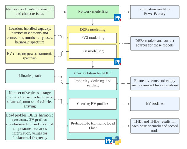
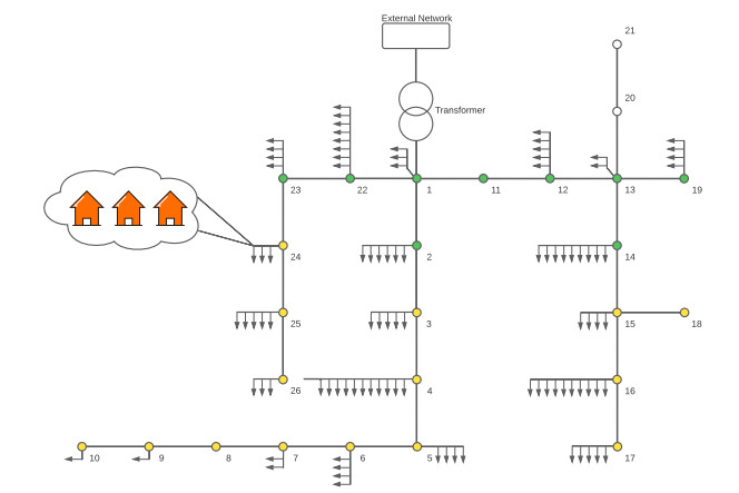
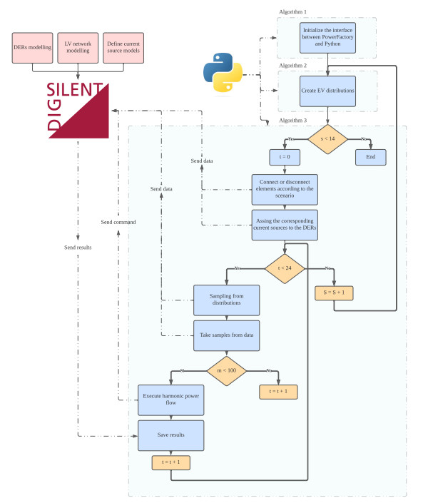
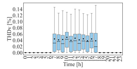
The integration of distributed energy resources (DERs) and, therefore, power electronic devices into distribution networks leads to harmonic distortion injection. However, studying harmonic distortion solely through deterministic approaches presents challenges due to the inherent random behavior of DERs. This study introduced a strategy that leverages PowerFactory's harmonic load flow tool. By combining it with Python co-simulation, probabilistic load flows can be developed. These load flows utilize current sources to represent harmonic distortion emitters with predefined harmonic spectra. The proposed strategy was implemented on a real network, where two different capacities of DERs were integrated at various locations within the network. The distributions for the total harmonic distortion of voltage ($ THD_{v} $) and the total harmonic distortion of current ($ THD_{i} $) were obtained 24 hours a day in nodes and lines of the network. The procedure allowed considering the uncertainty associated to the DERs integration in distribution networks in the study of harmonic distortion, which, speaking from a simulation approach, is scarce in the literature.
Citation: Cristian Cadena-Zarate, Juan Caballero-Peña, German Osma-Pinto. Simulation-based probabilistic-harmonic load flow for the study of DERs integration in a low-voltage distribution network[J]. AIMS Electronics and Electrical Engineering, 2024, 8(1): 53-70. doi: 10.3934/electreng.2024003
The integration of distributed energy resources (DERs) and, therefore, power electronic devices into distribution networks leads to harmonic distortion injection. However, studying harmonic distortion solely through deterministic approaches presents challenges due to the inherent random behavior of DERs. This study introduced a strategy that leverages PowerFactory's harmonic load flow tool. By combining it with Python co-simulation, probabilistic load flows can be developed. These load flows utilize current sources to represent harmonic distortion emitters with predefined harmonic spectra. The proposed strategy was implemented on a real network, where two different capacities of DERs were integrated at various locations within the network. The distributions for the total harmonic distortion of voltage ($ THD_{v} $) and the total harmonic distortion of current ($ THD_{i} $) were obtained 24 hours a day in nodes and lines of the network. The procedure allowed considering the uncertainty associated to the DERs integration in distribution networks in the study of harmonic distortion, which, speaking from a simulation approach, is scarce in the literature.

| [1] | IRENA (2019) Innovation landscape for a renewable-powered future: Solutions to integrate variable renewables. International Renewable Energy Agency, Abu Dhabi. Available from: https://www.irena.org/publications/2019/Feb/Innovation-landscape-for-a-renewable-powered-future. |
| [2] | IRENA (2020) Energy Transition. Available from: https://www.irena.org/energytransition. |
| [3] |
Caballero-Peña J, Cadena-Zarate C, Osma-Pinto G (2023) Hourly characterization of the integration of DER in a network from deterministic and probabilistic approaches using Co-simulation PowerFactory-Python. Alex Eng J 63: 283–305. https://doi.org/10.1016/j.aej.2022.08.005. doi: 10.1016/j.aej.2022.08.005

|
| [4] |
Zhi H, Zhang M, Li R, Zhao J, Wang J, Li X, et al. (2021) A Power-based Piecewise Probabilistic Harmonic Model of Secondary Residential System. 2021 IEEE 5th Conference on Energy Internet and Energy System Integration (EI2), 1175–1179. https://doi.org/10.1109/EI252483.2021.9713235 doi: 10.1109/EI252483.2021.9713235
|
| [5] |
Galvani S, Hagh MT, Sharifian MBB, Mohammadi-Ivatloo B (2019) Multiobjective Predictability-Based Optimal Placement and Parameters Setting of UPFC in Wind Power Included Power Systems. IEEE T Ind Inform 15: 878–888. https://doi.org/10.1109/TII.2018.2818821 doi: 10.1109/TII.2018.2818821
|
| [6] |
Xie X, Sun Y (2022) A piecewise probabilistic harmonic power flow approach in unbalanced residential distribution systems. International Journal of Electrical Power and Energy Systems 141: 108114. https://doi.org/10.1016/j.ijepes.2022.108114 doi: 10.1016/j.ijepes.2022.108114
|
| [7] |
Nasrfard-Jahromi F, Mohammadi M (2016) Probabilistic harmonic load flow using an improved kernel density estimator. International Journal of Electrical Power and Energy Systems 78: 292–298. https://doi.org/10.1016/j.ijepes.2015.11.076 doi: 10.1016/j.ijepes.2015.11.076
|
| [8] |
Mohammadi M. (2015) Probabilistic harmonic load flow using fast point estimate method. IET Generation, Transmission and Distribution 9: 1790–1799. https://doi.org/10.1049/iet-gtd.2014.0669 doi: 10.1049/iet-gtd.2014.0669
|
| [9] |
Palomino A, Parvania M (2020) Data-Driven Risk Analysis of Joint Electric Vehicle and Solar Operation in Distribution Networks. IEEE Open Access Journal of Power and Energy 7: 141–150. https://doi.org/10.1109/oajpe.2020.2984696 doi: 10.1109/oajpe.2020.2984696
|
| [10] |
Yan J, Zhang J, Liu Y, Lv G, Han S, Alfonzo IEG (2020) EV charging load simulation and forecasting considering traffic jam and weather to support the integration of renewables and EVs. Renew Energ 159: 623–641. https://doi.org/10.1016/j.renene.2020.03.175 doi: 10.1016/j.renene.2020.03.175
|
| [11] |
Hemmatpour MH, Rezaeian Koochi MH, Dehghanian P, Dehghanian P (2022) Voltage and energy control in distribution systems in the presence of flexible loads considering coordinated charging of electric vehicles. Energy 239: 121880. https://doi.org/10.1016/j.energy.2021.121880 doi: 10.1016/j.energy.2021.121880
|
| [12] |
Alzahrani A, Alharthi H, Khalid M (2020) Minimization of Power Losses through Optimal Battery Placement in a Distributed Network with High Penetration of Photovoltaics. Energies 13: Article Number 140. https://doi.org/10.3390/en13010140 doi: 10.3390/en13010140
|
| [13] |
Schneider KP, Mather BA, Pal BC, Ten CW, Shirek GJ, Zhu H, et al. (2018) Analytic Considerations and Design Basis for the IEEE Distribution Test Feeders. IEEE T Power Syst 33: 3181–3188. https://doi.org/10.1109/TPWRS.2017.2760011 doi: 10.1109/TPWRS.2017.2760011
|
| [14] |
Galvani S, Rezaeian Marjani S, Morsali J, Ahmadi Jirdehi M (2019) A new approach for probabilistic harmonic load flow in distribution systems based on data clustering. Electr Power Syst Res 176: 105977. https://doi.org/10.1016/j.epsr.2019.105977 doi: 10.1016/j.epsr.2019.105977
|
| [15] |
Xie X, Peng F, Zhang Y (2022) A data-driven probabilistic harmonic power flow approach in power distribution systems with PV generations. Appl Energy 321: 119331. https://doi.org/10.1016/j.apenergy.2022.119331 doi: 10.1016/j.apenergy.2022.119331
|
| [16] |
Ma Y, Azuatalam D, Power T, Chapman AC, Verbič G (2019) A novel probabilistic framework to study the impact of photovoltaic-battery systems on low-voltage distribution networks. Appl Energy 254: 113669. https://doi.org/10.1016/j.apenergy.2019.113669 doi: 10.1016/j.apenergy.2019.113669
|
| [17] |
Lehtonen M (1998) A method for probabilistic harmonic load-flow analysis in power systems. Eur T Electr Power 8: 47–50. https://doi.org/10.1002/etep.4450080108 doi: 10.1002/etep.4450080108
|
| [18] |
Russo A, Varilone P, Caramia P (2014) Point estimate schemes for probabilistic harmonic power flow. 2014 16th International Conference on Harmonics and Quality of Power (ICHQP), 19–23. https://doi.org/10.1109/ICHQP.2014.6842890 doi: 10.1109/ICHQP.2014.6842890
|
| [19] |
Yu G, Lin T (2016) 2m+1 point estimate method for probabilistic harmonic power flow. 2016 IEEE Power and Energy Society General Meeting (PESGM), 1–5. https://doi.org/10.1109/PESGM.2016.7741657 doi: 10.1109/PESGM.2016.7741657
|
| [20] |
Ismael SM, Abdel Aleem SHE, Abdelaziz AY, Zobaa AF (2019) Probabilistic Hosting Capacity Enhancement in Non-Sinusoidal Power Distribution Systems Using a Hybrid PSOGSA Optimization Algorithm. Energies 12: Article Number 1018. https://doi.org/10.3390/en12061018 doi: 10.3390/en12061018
|
| [21] |
Gandoman FH, Sharaf AM, Abdel Aleem SHE, Jurado F (2017) Distributed FACTS stabilization scheme for efficient utilization of distributed wind energy systems. Int T Electr Energy 27: e2391. https://doi.org/10.1002/etep.2391 doi: 10.1002/etep.2391
|
| [22] |
Martínez-Peñaloza A, Osma-Pinto G (2021) Analysis of the performance of the Norton equivalent model of a photovoltaic system under different operating scenarios. Int Rev Electr Eng 16: 328–343. https://doi.org/10.15866/iree.v16i4.20278 doi: 10.15866/iree.v16i4.20278
|
| [23] |
Caro L, Ramos G, Montenegro D, Celeita D (2020) Variable Harmonic Distortion in Electric Vehicle Charging Stations. 2020 IEEE Industry Applications Society Annual Meeting, 1–6. https://doi.org/10.1109/IAS44978.2020.9334798 doi: 10.1109/IAS44978.2020.9334798
|
| [24] |
Angelim JH, Affonso CD (2019) Probabilistic Impact Assessment of Electric Vehicles Charging on Low Voltage Distribution Systems. 2019 IEEE PES Innovative Smart Grid Technologies Conference - Latin America (ISGT Latin America), 1–6. https://doi.org/10.1109/ISGT-LA.2019.8895494 doi: 10.1109/ISGT-LA.2019.8895494
|
| [25] |
Prusty BR, Jena D (2017) A critical review on probabilistic load flow studies in uncertainty constrained power systems with photovoltaic generation and a new approach. Renew Sust Energy Rev 69: 1286–1302. https://doi.org/10.1016/j.rser.2016.12.044 doi: 10.1016/j.rser.2016.12.044
|
| [26] | Jahic A, Eskander M, Schulz D (2019) Bus depot simulator: Steady-state python and digsilent co-simulation for large-scale electric bus depots. NEIS 2019 - Conference on Sustainable Energy Supply and Energy Storage Systems, 85–91. |
Figures(9) / Tables(1)

Cristian Cadena-Zarate, Juan Caballero-Peña, German Osma-Pinto. Simulation-based probabilistic-harmonic load flow for the study of DERs integration in a low-voltage distribution network[J]. AIMS Electronics and Electrical Engineering, 2024, 8(1): 53-70. doi: 10.3934/electreng.2024003


 DownLoad: