This study uses laminar and turbulent flow models to investigate the blood flow dynamics in a specific carotid bifurcation. Pulsatile boundary conditions and the rigid carotid artery wall are considered. Three viscosity models describe the non-Newtonian blood behavior. The Fluent solver and the finite volume method solve the equations. Results show a Poiseuille-like flow in the common carotid artery (CCA), unaffected by the flow regime, viscosity model, or boundary conditions. The branching zone exhibits a C-shaped stagnation zone with low velocity and wall shear stress due to the CCA widening and ICA/ECA curvature. Strong secondary flow is observed in the carotid sinus; the flow is directed towards the inner wall with higher velocity in the internal carotid artery. Discrepancies between viscosity models are pronounced in laminar flow, particularly with the natural boundary conditions. The non-Newtonian blood behavior is more apparent in the laminar flow of the external carotid artery, especially with the second set of boundary conditions.
Citation: Boukedjane Mouloud, Bahi Lakhdar. Characterizing pulsatile blood flow in a specific carotid bifurcation: insights into hemodynamics and rheology models[J]. AIMS Biophysics, 2023, 10(3): 281-316. doi: 10.3934/biophy.2023019
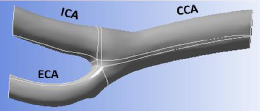
This study uses laminar and turbulent flow models to investigate the blood flow dynamics in a specific carotid bifurcation. Pulsatile boundary conditions and the rigid carotid artery wall are considered. Three viscosity models describe the non-Newtonian blood behavior. The Fluent solver and the finite volume method solve the equations. Results show a Poiseuille-like flow in the common carotid artery (CCA), unaffected by the flow regime, viscosity model, or boundary conditions. The branching zone exhibits a C-shaped stagnation zone with low velocity and wall shear stress due to the CCA widening and ICA/ECA curvature. Strong secondary flow is observed in the carotid sinus; the flow is directed towards the inner wall with higher velocity in the internal carotid artery. Discrepancies between viscosity models are pronounced in laminar flow, particularly with the natural boundary conditions. The non-Newtonian blood behavior is more apparent in the laminar flow of the external carotid artery, especially with the second set of boundary conditions.

| [1] |
Basmadjian D (1989) Embolization: critical thrombus height, shear rates, and pulsatility. Patency of blood vessels. J Biomed Mater Res Part A 23: 1315-1326. https://doi.org/10.1002/jbm.820231108 
|
| [2] | Cao P, Duhamel Y, Olympe G, et al. (2013) A new production method of elastic silicone carotid phantom based on MRI acquisition using rapid prototyping technique. In: 35th Ann Int Conf IEEE Eng Med Biol Soc (EMBC) : 5331-5334. https://doi.org/10.1109/EMBC.2013.6610753 |
| [3] |
Cibis M, Potters VW, Selwaness M, et al. (2016) Relation between wall shear stress and carotid artery wall thickening MRI versus CFD. J Biomech 49: 735-741. https://doi.org/10.1016/j.jbiomech.2016.02.004
|
| [4] |
Peiffer V, Sherwin SJ, Weinberg PD (2013) Does low and oscillatory wall shear stress correlate spatially with early atherosclerosis? A systematic review. Cardiovasc Res 99: 242-250. https://doi.org/10.1093/cvr/cvt044
|
| [5] |
Conti M, Long C, Marconi M, et al. (2016) Carotid artery hemodynamics before and after stenting: A patient-specific CFD study. Comput Fluids 141: 62-74. https://doi.org/10.1016/j.compfluid.2016.04.006
|
| [6] |
Berger SA, Jou LD (2000) Flows in stenotic vessels. Annu Rev Fluid Mech 32: 347-382. https://doi.org/10.1146/annurev.fluid.32.1.347
|
| [7] | Caro CG, Pedley TJ, Schroter RC, et al. (1978) The Mechanics of the Circulation. Oxford: Oxford University Press. |
| [8] |
Jeong W, Seong J (2014) Comparison of effects on technical variances of computational fluid dynamics (CFD) software based on finite element and finite volume methods. Int J Mech Sci 78: 19-26. https://doi.org/10.1016/j.ijmecsci.2013.10.017
|
| [9] | Algabri Y, Chatpun S, Taib I (2019) An investigation of pulsatile blood flow in an angulated neck of abdominal aortic aneurysm using computational fluid dynamics. J Adv Res Fluid Mech Therm Sci 57: 265-274. Retrieved from https://www.akademiabaru.com/submit/index.php/arfmts/article/view/2557 |
| [10] |
Lopes D, Puga H, Teixeira JC, et al. (2019) Influence of arterial mechanical properties on carotid blood flow: Comparison of CFD and FSI studies. Int J Mech Sci 160: 209-218. https://doi.org/10.1016/j.ijmecsci.2019.06.029
|
| [11] | Srivastava A CFD Simulation of Blood Flow through Carotid Artery Bifurcation with Stenosis (2017). Doctoral dissertation, Indian Inst Technol |
| [12] |
Sone S, Hyase T, Funamoto TK, et al. (2017) Photoplethysmography and ultrasonic measurement-integrated simulation to clarify the relation between two-dimensional unsteady blood flow field and forward and backward waves in a carotid artery. Med Biol Eng Comput 55: 719-731. https://doi.org/10.1007/s11517-016-1543-4
|
| [13] |
Kannojiya V, Das AK, Das PK (2020) Simulation of blood as fluid: A review from rheological aspects. IEEE Rev Biomed Eng 14: 327-341. https://doi.org/10.1109/RBME.2020.3011182
|
| [14] | Trigui A, Ben Chiekh M, Bera JC Simulation numérique de l'interaction fluide-structure dans les artères sténosées (2017). IEES-2017, Djerba, Tunisia |
| [15] |
Bit A, Chattopadhyay H (2014) Assessment of rheological models for prediction of transport phenomena in stenosed artery. Prog Comput Fluid Dyn 14: 363-374. https://doi.org/10.1504/PCFD.2014.065468
|
| [16] | Kleinstreuer C (2006) Biofluid Dynamics: Principles and Selected Applications. New York: CRC Press. |
| [17] |
Pedley JT (1980) The Fluid Mechanics of Large Blood Vessels. Cambridge: Cambridge University Press. https://doi.org/10.1017/CBO9780511896996
|
| [18] |
Ling CS, Atabek BH (1972) A nonlinear analysis of pulsatile flow in arteries. J Fluid Mech 55: 493-511. https://doi.org/10.1017/S0022112072001971
|
| [19] | Burton CA (1966) Physiology and Biophysics of the Circulation: Introductory Text. Chicago: Year Book Medical Publisher. |
| [20] |
Mandal PK, Chakravarty S, Mandal A (2007) Numerical study of the unsteady flow of non-Newtonian fluid through differently shaped arterial stenoses. Int J Comput Math 84: 1059-1077. https://doi.org/10.1080/00207160701288881
|
| [21] |
Tabakova S, Raynov P, Nikolov N (2017) Newtonian and non-Newtonian pulsatile blood flow in arteries with model aneurysms. Advanced Computing in Industrial Mathematics . Cham: Springer 187-197. https://doi.org/10.1007/978-3-319-49544-6_16
|
| [22] | Vasava P, Jalali P, Dabagh M, et al. (2011) Finite element modelling of pulsatile blood flow in idealized model of human aortic arch: Study of hypotension and hypertension. Comput Math Methods Med 2012: 14. https://doi.org/10.1155/2012/861837 |
| [23] |
Conlon MJ, Russell DL, Mussivand T (2006) Development of a mathematical model of the human circulatory system. Ann Biomed Eng 34: 1400-1413. https://doi.org/10.1007/s10439-006-9164-y
|
| [24] | Patankar SV (1980) Numerical Heat Transfer and Fluid Flow. New York: Hemisphere Publ. Corp. 288. https://doi.org/10.1201/9781482234213 |
| [25] | Mamuna K, Funazakia K (2020) Comparative study of non-Newtonian physiological blood flow through the elastic stenotic artery with rigid wall stenotic artery. Ser Biomech 34: 43-58. |
| [26] |
Joshi AK, Leask RI, Myers JG, et al. (2004) Intimal thickness is not associated with wall shear stress patterns in the human right coronary artery. Arterioscler Thromb Vasc Biol 24: 2408-2413. https://doi.org/10.1161/01.ATV.0000147118.97474.4b
|
| [27] |
Fry DL (1968) Acute vascular endothelial changes associated with increased blood velocity gradients. Circ Res 22: 165-197. https://doi.org/10.1161/01.RES.22.2.165
|
| [28] |
Savabi R, Nabaei M, Farajollahi S, et al. (2020) Fluid structure interaction modeling of aortic arch and carotid bifurcation. Int J Mech Sci 165: 105222. https://doi.org/10.1016/j.ijmecsci.2019.105222
|
| [29] |
Lopes D, Agujetas R, Puga H, et al. (2021) Analysis of finite element and finite volume methods for fluid-structure interaction simulation of blood flow in a real stenosed artery. Int J Mech Sci 207: 106650. https://doi.org/10.1016/j.ijmecsci.2021.106650
|
| [30] |
De Wilde D, Trachet B, De Meyer G, et al. (2016) The influence of anesthesia and fluid-structure interaction on simulated shear stress patterns in the carotid bifurcation of mice. J Biomech 49: 2741-2747. https://doi.org/10.1016/j.jbiomech.2016.06.010
|
| [31] |
Malek AM, Alper SI, Izumo S (1999) Hemodynamic shear stress and its role in atherosclerosis. JAMA 282: 2035-2042. https://doi:10.1001/jama.282.21.2035
|
| [32] | Ku DN, Giddens DP, Zarins CK, et al. (1985) Pulsatile flow and atherosclerosis in human carotid bifurcation: positive correlation between plaque location and low and oscillating shear stress. Arterioscler Thromb Vasc Biol 5: 293-302. https://doi.org/10.1161/01.ATV.5.3.293 |
| [33] |
Shaaban AM, Duerinckx AJ (2000) Wall shear stress and early atherosclerosis: a review. Am J Roentgenol 174: 1657-1665. https://doi.org/10.2214/ajr.174.6.1741657
|
| [34] |
Boyd J, Buick J, Cosgrove JA, et al. (2000) Application of the lattice Boltzmann model to simulated stenosis growth in a two-dimensional carotid artery. Phys Med Biol 50: 4783. https://doi.org/10.1088/0031-9155/50/20/003
|
| [35] | Buchmann NA, Jermy MC (2008). Blood flow measurements in idealised and patient-specific models of the human carotid artery. Proc 14th Int Symp Appl Laser Tech Fluid Mech, Lisbon, Portugal |
| [36] |
Apostolidis AJ, Moyer AP, Beris AN (2016) Non-Newtonian effects in blood flow simulations of coronary arterial flow. J Nonnewton Fluid Mech 233: 155-165. https://doi.org/10.1016/j.jnnfm.2016.03.008
|


Figures(69) / Tables(5)

Boukedjane Mouloud, Bahi Lakhdar. Characterizing pulsatile blood flow in a specific carotid bifurcation: insights into hemodynamics and rheology models[J]. AIMS Biophysics, 2023, 10(3): 281-316. doi: 10.3934/biophy.2023019


 DownLoad: