In this essay, we have presented a fractional numerical model of breast cancer stages with cardiac outcomes. Five compartments were used to build the model, each of which represented a subpopulation of breast cancer patients. Variables A, B, C, D, and E each represent a certain subpopulation. They are levels 1 and 2 (A), level 3 (B), level 4 (C), disease-free (D) and cardiotoxic (E). We have demonstrated that the fractional model has a stable solution. We also discuss how to optimally control this model and numerically simulate the control problem. Using numerical simulations, we computed the results of the dissection. The model's compartment diagram has been completed. A predictor-corrector method has been used to manage the fractional derivatives and produce numerical solutions. The Caputo sense has been used to describe fractional derivatives. The results have been illustrated through numerical simulations. Furthermore, the numerical simulations show that the cancer breast malignant growth fractional order model is easier to model than the traditional integer-order model. To compute the results, we have used mathematical programming. We have made it clear that the numerical method that was applied in this publication to solve this model was not utilized by any other author before that, nor has this method been investigated in the past. Our investigation established this approach.
Citation: Shaimaa A. M. Abdelmohsen, D. Sh. Mohamed, Haifa A. Alyousef, M. R. Gorji, Amr M. S. Mahdy. Mathematical modeling for solving fractional model cancer bosom malignant growth[J]. AIMS Biophysics, 2023, 10(3): 263-280. doi: 10.3934/biophy.2023018
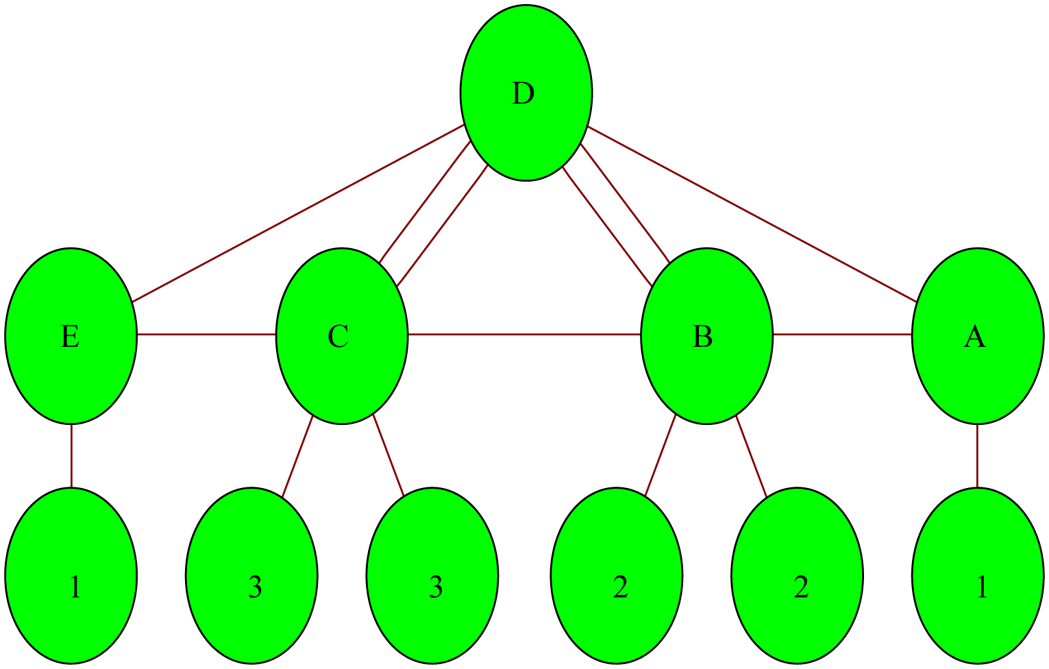
In this essay, we have presented a fractional numerical model of breast cancer stages with cardiac outcomes. Five compartments were used to build the model, each of which represented a subpopulation of breast cancer patients. Variables A, B, C, D, and E each represent a certain subpopulation. They are levels 1 and 2 (A), level 3 (B), level 4 (C), disease-free (D) and cardiotoxic (E). We have demonstrated that the fractional model has a stable solution. We also discuss how to optimally control this model and numerically simulate the control problem. Using numerical simulations, we computed the results of the dissection. The model's compartment diagram has been completed. A predictor-corrector method has been used to manage the fractional derivatives and produce numerical solutions. The Caputo sense has been used to describe fractional derivatives. The results have been illustrated through numerical simulations. Furthermore, the numerical simulations show that the cancer breast malignant growth fractional order model is easier to model than the traditional integer-order model. To compute the results, we have used mathematical programming. We have made it clear that the numerical method that was applied in this publication to solve this model was not utilized by any other author before that, nor has this method been investigated in the past. Our investigation established this approach.

| [1] |
Fitzmaurice C, Dicker D, Pain A, et al. (2015) The global burden of cancer 2013. JAMA Oncol 1: 505-527. https://doi:10.1001/jamaoncol.2015.0735 
|
| [2] |
Vasiliadis I, Kolovou G, Mikhailidis DP (2014) Cardiotoxicity and cancer therapy. Angiology 65: 369-371. https://doi.org/10.1177/0003319713498298
|
| [3] |
Mercurio V, Pirozzi F, Lazzarini E, et al. (2016) Models of heart failure based on the cardiotoxicity of anticancer drugs. J Card Fail 22: 449-458. https://doi.org/10.1016/j.cardfail.2016.04.008
|
| [4] |
Byrne HM (2010) Dissecting cancer through mathematics: from the cell to the animal model. Nat Rev Cancer 10: 221-230. https://doi.org/10.1038/nrc2808
|
| [5] | Fathoni M, Gunardi G, Kusumo FA, et al. (2019) Mathematical model analysis of breast cancer stages with side effects on heart in Chemotherapy patients. AIP Conference Proceedings 2192: 1-9. https://doi.org/10.1063/1.5139153 |
| [6] |
Mohamed SM, Elagan SK, Almalki SJ, et al. (2022) Optimal control and solving of cellular DNA cancer model. Appl Math Inform Sci 16: 109-119. http://dx.doi.org/10.18576/amis/160111?
|
| [7] |
Mahdy AMS, Lotfy K, El-Bary AA (2022) Use of optimal control in studying the dynamical behaviors of fractional financial awareness models. Soft Comput 26: 3401-3409. https://doi.org/10.1007/s00500-022-06764-y
|
| [8] | Mahdy AMS (2023) Stability existence and uniqueness for solving fractional glioblastoma multiforme using a Caputo–Fabrizio derivative. Math Method Appl Sci : 1-18. https://doi.org/10.1002/mma.9038 |
| [9] |
Higazy M, El-Mesady A, et al. (2021) Numerical approximate solutions, and optimal control on the deathly Lassa Hemorrhagic fever disease in pregnant women. J Funct Spaces 2021: 1-15. https://doi.org/10.1155/2021/2444920
|
| [10] |
Mahdy AMS, Gepreel KA, Lotfy K, et al. (2023) Reduced differential transform and Sumudu transform methods for solving fractional financial models of awareness. Appl Math J Chinese Univ 38: 338-356. https://doi.org/10.1007/s11766-023-3713-0
|
| [11] |
Agrawal OP (2002) Formulation of Euler-Lagrange equations for fractional variational problems. J Math Anal Appl 272: 368-379. https://doi.orgS0022-247X(02)00180-4
|
| [12] | Agrawal OP (2006) A formulation and numerical scheme for fractional optimal control problems. IFAC Proc 39: 68-72. https://doi.org/10.3182/20060719-3-PT-4902.00011 |
| [13] |
Agrawal OP, Defterli O, Baleanu D (2010) Fractional optimal control problems with several state and control variables. J Vib Control 16: 1967-1976. https://doi.org/10.1177/1077546309353361
|
| [14] | Mahdy AMS (2022) A numerical method for solving the nonlinear equations of Emden-Fowler models. J Ocean Eng Sci . In Press. https://doi.org/10.1016/j.joes.2022.04.019 |
| [15] |
Sweilam NH, Al-Mekhlafi SM (2018) Optimal control for a nonlinear mathematical model of tumor under immune suppression: a numerical approach. Optimal Control Appl Method 39: 1581-1596. https://doi.org/10.1002/oca.2427
|
| [16] |
Sweilam NH, Al-Mekhlafi SM, Baleanu D (2019) Optimal control for a fractional tuberculosis infection model including the impact of diabetes and resistant strains. J Adv Res 17: 125-137. https://doi.org/10.1016/j.jare.2019.01.007
|
| [17] |
Sweilam NH, Saad OM, Mohamed DG (2019) Fractional optimal control in transmission dynamics of West Nile model with state and control time delay a numerical approach. Adv Differ Equ 2019: 1-25. https://doi.org/10.1186/s13662-019-2147-8
|
| [18] | Sweilam NH, Saad OM, Mohamed DG (2019) Numerical treatments of the tranmission dynamics of West Nile virus and it's optimal control. Electonic J Mat Anal Appl 7: 9-38. https://doi.org/10.21608/ejmaa.2019.312771 |
| [19] |
Abaid Ur Rehman M, Ahmad J, Hassan A, et al. (2022) The dynamics of a fractional order mathematical model of cancer Ttumor disease. Symmetry 14: 1694. https://doi.org/10.3390/sym14081694
|
| [20] |
Alotaibi H, Gepreel KA, Mohamed SM, et al. (2022) An approximate numerical methods for mathematical and physical studies for covid-19 models. Comput Syst Sci Eng 42: 1147-1163. https://doi.org/10.32604/csse.2022.020869
|
| [21] |
Wise SM, Lowengrub JS, Frieboes HB, et al. (2008) Three-dimensional multispecies nonlinear tumor growth-I: model and numerical method. J Theor Biol 253: 524-543. https://doi.org/doi: 10.1016/j.jtbi.2008.03.027
|
| [22] | Moyo S, Leach PGL (2004) Symmetry methods applied to a mathematical model of a tumour of the brain. Proceedings of Institute of Mathematics of NAS of Ukraine 50: 204-210. |
| [23] |
El-Saka HAA (2014) The fractional order SIS epidemic model with variable population size. J Egypt Mathematical Soc 22: 50-54. https://doi.org/10.1016/j.joems.2013.06.006
|
| [24] |
Iyiola OS, Zaman FD (2014) A fractional diffusion equation model for cancer tumor. AIP Adv 4: 107121. https://doi.org/10.1063/1.4898331
|
| [25] |
Mahdy AMS, Mohamed SM, Al Amiri AY, et al. (2022) Optimal control and spectral collocation method for solving smoking models. Intell Autom Soft Comput 31: 899-915. https://doi.org/10.32604/iasc.2022.017801
|
| [26] | Mahdy AMS, Mohamed MS, Lotfy K, et al. (2021) Numerical solution and dynamical behaviors for solving fractional nonlinear rubella ailment disease model. Results Phys 24: 1-10. https://doi.org/10.1016/j.rinp.2021.104091 |
| [27] |
Gepreel KA, Mohamed MS, Alotaibi H, et al. (2021) Dynamical behaviors of nonlinear Coronavirus (COVID-19) model with numerical studies. Comput Mater Continua 67: 675-686. https://doi.org/10.32604/cmc.2021.012200
|
| [28] |
Ahmed N, Shah NA, Ali F, et al. (2021) Analytical solutions of the fractional mathematical model for the concentration of tumor cells for constant killing rate. Mathematics 9: 1156. https://doi.org/10.3390/math9101156
|
| [29] |
Sabir Z, Munawar M, Abdelkawy MA, et al. (2022) Numerical investigations of the fractional-order mathematical model underlying immune chemotherapeutic treatment for breast cancer using the neural networks. Fractal Fract 6: 184. https://doi.org/10.3390/fractalfract6040184
|
| [30] | Maddalena L, Ragni S (2020) Existence of solutions and numerical approximation of a non-local tumor growth model. Math Med Biol A J IMA 37: 58-82. https://doi.10.1093/imammb/dqz005 |
| [31] |
Kolev M, Zubik KB (2011) Numerical solutions for a model of tissue invasion and migration of tumour cells. Comput Math Methods Med 2011: 452320. https://doi.org/10.1155/2011/452320
|
| [32] | Ismail GM, Mahdy AMS, Amer YA, et al. (2022) Computational simulations for solving nonlinear composite oscillation fractional. J Ocean Eng Sci : 1-10. https://doi.org/10.1016/j.joes.2022.06.029 |
| [33] |
Yasir M, Ahmad S, Ahmed F, et al. (2017) Improved numerical solutions for chaotic-cancer-model. AIP Adv 7: 015110. https://doi.org/10.1063/1.4974881
|
| [34] | Mahdy AMS, Amer YA, Mohamed MS, et al. (2020) General fractional financial models of awareness with Caputo Fabrizio derivative. Adv Mechan Eng 12: 1-9. https://doi.org/10.1177/1687814020975525 |
| [35] |
Diethelm K, Ford NJ, Freed AD, et al. (2005) Algorithms for the fractional calculus: a selection of numerical methods. Comput Meth Appl Mech Eng 194: 743-773. https://doi.org/10.1016/j.cma.2004.06.006
|
| [36] |
Li YX, Wei M, Tong S (2022) Event triggered adaptive neural control for fractional order nonlinear systems based on finitetime scheme. IEEE T Cybernetics 52: 9481-9489. https://doi.org/10.1109/TCYB.2021.3056990
|
| [37] |
Wei M, Li YX, Tong S (2020) Event-triggered adaptive neural control of fractional-order nonlinear systems with full-state constraints. Neurocomputing 412: 320-326. https://doi.org/10.1016/j.neucom.2020.06.082
|
| [38] |
Li YX (2020) Barrier Lyapunov function-based adaptive asymptotic tracking of nonlinear systems with unknown virtual control coefficients. Automatica 121: 109181. https://doi.org/10.1016/j.automatica.2020.109181
|
| [39] |
Solís-Pérez JE, Gómez-Aguilar JF, Atangana A (2019) A fractional mathematical model of breast cancer competition model. Chaos, Soliton Fract 127: 38-54. https://doi.org/10.1016/j.chaos.2019.06.027
|
| [40] |
Diethelm K, Ford NJ, Freed AD (2002) A predictor-corrector approach for the numerical solution of fractional differential equations. Nonlinear Dyamics 29: 3-22. https://doi.org/10.1023/A:1016592219341
|
| [41] |
Diethelm K, Ford NJ, Freed AD (2004) Detailed error analysis for a fractional adams method. Numer Algorithms 36: 31-52. https://doi.org/10.1023/B:NUMA.0000027736.85078.be
|


Figures(3) / Tables(1)

Shaimaa A. M. Abdelmohsen, D. Sh. Mohamed, Haifa A. Alyousef, M. R. Gorji, Amr M. S. Mahdy. Mathematical modeling for solving fractional model cancer bosom malignant growth[J]. AIMS Biophysics, 2023, 10(3): 263-280. doi: 10.3934/biophy.2023018


 DownLoad: