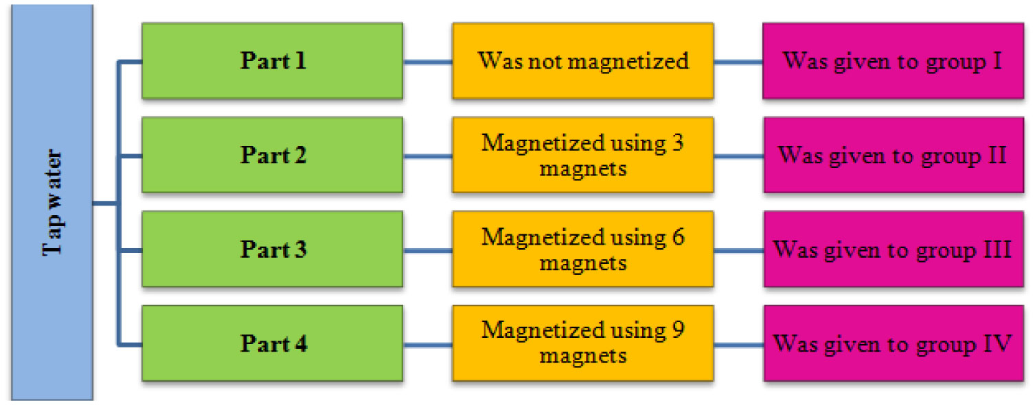
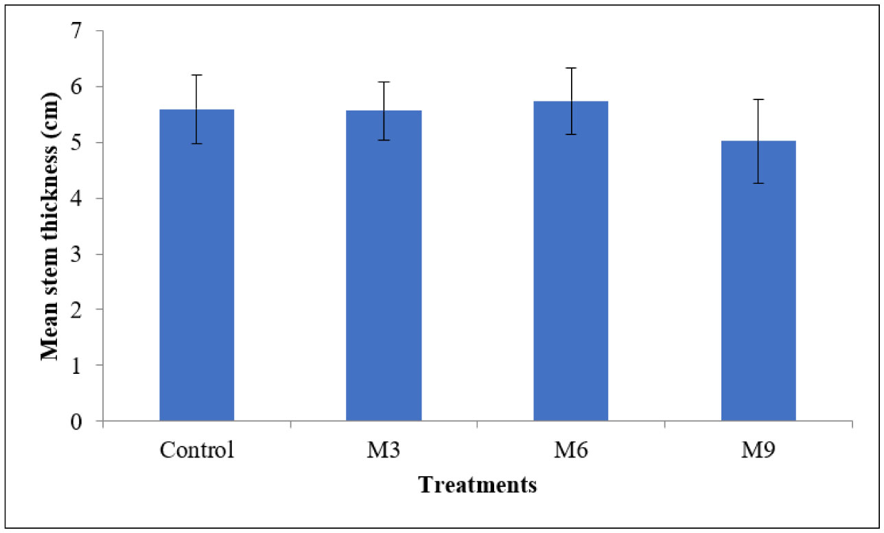
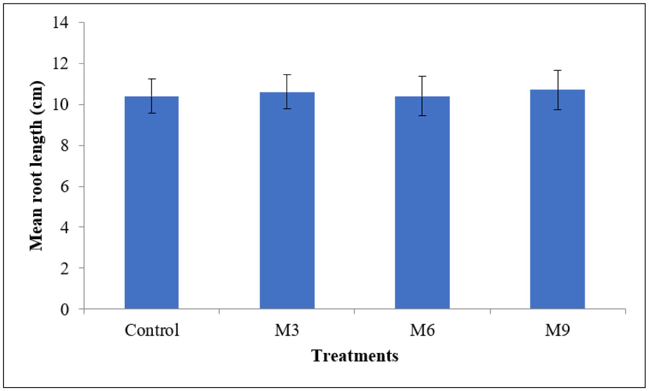
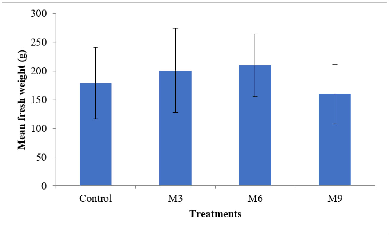
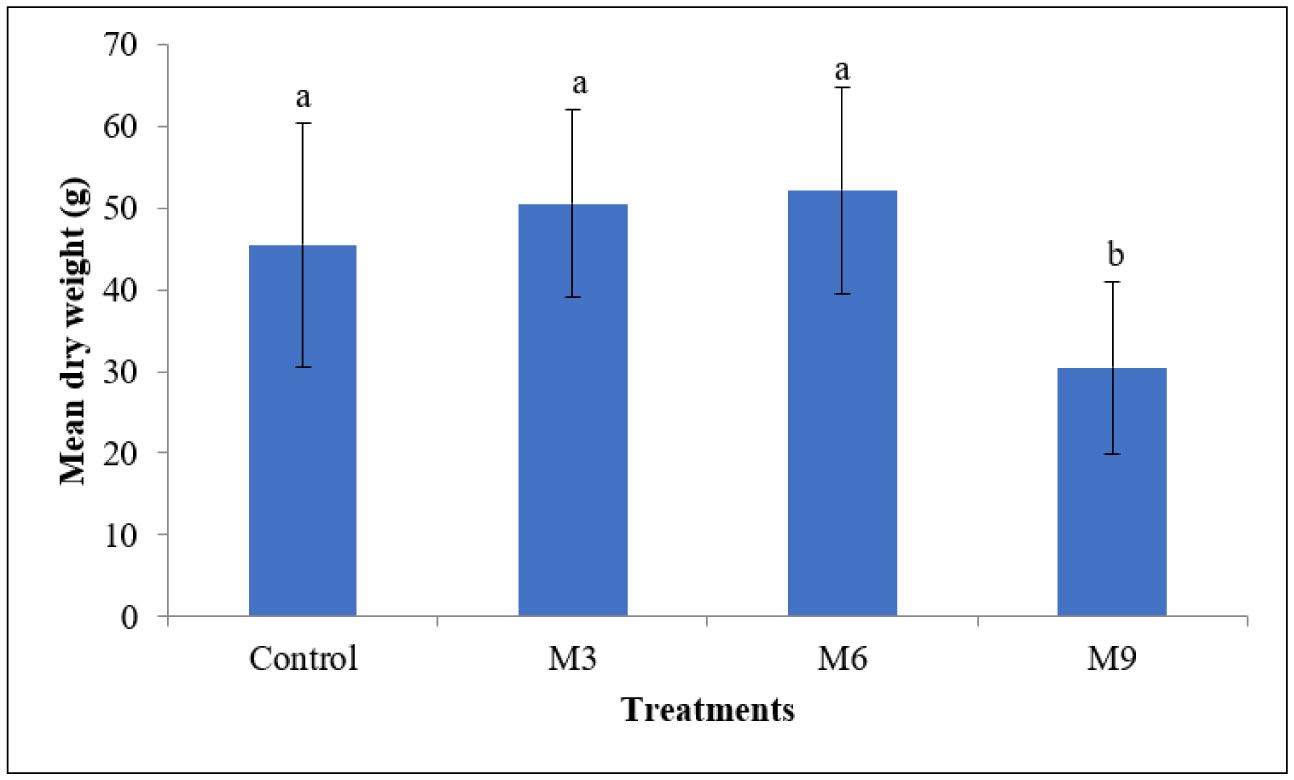
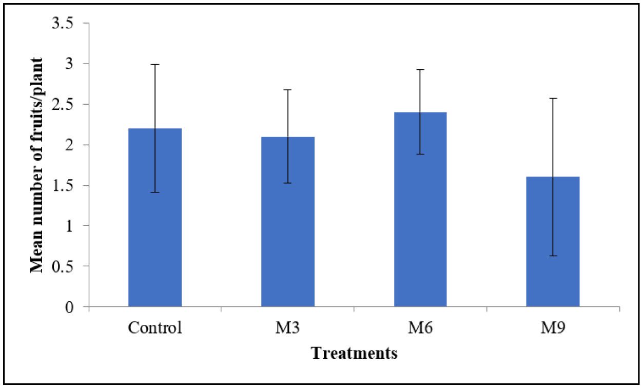
The current study presents the investigation of the effects of magnetic water treatment on the growth of corn (Zea mays) plants. A total of 120 corn seeds were divided into four groups in a complete randomized design. Normal tap water was taken and divided into four parts. The first group was given non-magnetized water, whereas the remaining three groups were given water magnetized with 3, 6 and 9 permanent magnets respectively. Eighteen permanent magnets (70 mT) and 4 pipes were used for this system. The results showed that the corn plants watered with magnetized water had higher shoot length than those of normal tap water. Magnetized water significantly increased the dry weight of corn plants when compared with the non-magnetized plants. The results revealed that magnetizing water with 6 magnets was the most influential in increasing the length of plants (194.10 ± 66.74 cm) and dry weight (52.22 ± 12.63 g). On the other hand, root length, stem thickness, and fresh weight were not significantly affected by magnetized water. The influence of magnetized water depends on the number of magnets used to magnetizing water. So as a clean and safe method, watering with magnetized water can be used to improve the growth parameters of the exposed plant.
Citation: Etimad Alattar, Khitam Elwasife, Eqbal Radwan. Effects of magnetic field treated water on some growth parameters of corn (Zea mays) plants[J]. AIMS Biophysics, 2021, 8(3): 267-280. doi: 10.3934/biophy.2021021
The current study presents the investigation of the effects of magnetic water treatment on the growth of corn (Zea mays) plants. A total of 120 corn seeds were divided into four groups in a complete randomized design. Normal tap water was taken and divided into four parts. The first group was given non-magnetized water, whereas the remaining three groups were given water magnetized with 3, 6 and 9 permanent magnets respectively. Eighteen permanent magnets (70 mT) and 4 pipes were used for this system. The results showed that the corn plants watered with magnetized water had higher shoot length than those of normal tap water. Magnetized water significantly increased the dry weight of corn plants when compared with the non-magnetized plants. The results revealed that magnetizing water with 6 magnets was the most influential in increasing the length of plants (194.10 ± 66.74 cm) and dry weight (52.22 ± 12.63 g). On the other hand, root length, stem thickness, and fresh weight were not significantly affected by magnetized water. The influence of magnetized water depends on the number of magnets used to magnetizing water. So as a clean and safe method, watering with magnetized water can be used to improve the growth parameters of the exposed plant.

| [1] | Alattar EM, Elwasife KY, Radwan ES, et al. (2019) Influence of magnetized water on the growth of corn (Zea mays) seedlings. Rom J biophys 29: 39-50. |
| [2] |
Czaplicki Z, Matyjas-Zgondek E, Strzelecki S (2020) Dyeing of wool and woolen fabrics in magnetically treated water. J Nat Fibers 1-8. doi: 10.1080/15440478.2019.1711286

|
| [3] |
Bugatin J, Bondarenko N, Gak EZ, et al. (1999) Magnetic treatment of irrigation water: Experimental results and application conditions. Environ Sci Technol 33: 1280-1285. doi: 10.1021/es980172k
|
| [4] |
Pang XF, Deng B (2008) Investigation of changes in properties of water under the action of a magnetic field. Sci China Phys Mech 51: 1621-1632. doi: 10.1007/s11433-008-0182-7
|
| [5] | Othman A, Sohaili J, Supian NS (2019) A review: Methodologies review of magnetic water treatment as green approach of water pipeline system. Pertanika J Sci & Technol 27: 281-296. |
| [6] |
Inaba H, Saitou T, Tozaki K, et al. (2004) Effect of the magnetic field on the melting transition of H2O and D2O measured by a high resolution and supersensitive differential scanning calorimeter. J Appl Phys 96: 6127-6132. doi: 10.1063/1.1803922
|
| [7] |
Chang KT, Weng CI (2008) An investigation into the structure of aqueous NaCl electrolyte solutions under magnetic fields. Comp Mater Sci 43: 1048-1055. doi: 10.1016/j.commatsci.2008.02.020
|
| [8] | Alattar EM, Elwasife KY, Radwan ES, et al. (2017) Response of corn (Zea mays), basil (Ocimim basilicum) and eggplant (Solanum melongena) seedlings to Wi-Fi radiation. Rom J biophys 27: 137-150. |
| [9] | Alattar EM, Elwasife KY, Radwan ES, et al. (2018) Effect of microwave treated water on the growth of corn (Zea mays) and pepper (Capsicum annuum) seedlings. Rom J biophys 28: 115-124. |
| [10] |
Alattar E, Radwan E (2020) Investigation of the effects of radio frequency water treatment on some characteristics of growth in pepper (capsicum annuum) plants. Adv Biosci Biotechnol 11: 22-48. doi: 10.4236/abb.2020.112003
|
| [11] |
Chapin FS, Bloom, Field CB, et al. (1987) Plant responses to multiple environmental factors. Bioscience 37: 49-57. doi: 10.2307/1310177
|
| [12] |
Kozyrskyi V, Zablodskiy M, Savchenko V, et al. (2019) The Magnetic Treatment of Water Solutions and Seeds of Agricultural Crops. In Advanced Agro-Engineering Technologies for Rural Business Development IGI Global, 256-292. doi: 10.4018/978-1-5225-7573-3.ch010
|
| [13] |
Hasan MM, Alharby HF, Hajar AS, et al. (2019) The effect of magnetized water on the growth and physiological conditions of moringa species under drought stress. Pol J Environ Stud 8: 1145-1155. doi: 10.15244/pjoes/85879
|
| [14] |
Seron C, Rezende R, Lorenzoni MZ, et al. (2019) Irrigation with water deficit applying magnetic water on scarlet eggplant. J Neotrpical Agric 6: 21-28. doi: 10.32404/rean.v6i4.3809
|
| [15] |
Fatahi P, Hajnorouzi A, Afzalzadeh R (2019) Improvement in photocatalytic properties of synthesized nano-structured ZnO in magnetic water and in presence of static magnetic field. Physica B Condens 555: 133-138. doi: 10.1016/j.physb.2018.11.026
|
| [16] | El-Yazied AA, Shalaby OA, El-Gizawy AM, et al. (2011) Effect of magnetic field on seed germination and transplant growth of tomato. J Am Sci 7: 306-312. |
| [17] | Shahin MM, Mashhour AMA, Abd-Elhady ESE (2016) Effect of magnetized irrigation water and seeds on some water properties, growth parameter and yield productivity of cucumber plants. Curr Sci Int 5: 152-164. |
| [18] | Alvarez J, Carbonell V, Martinez E, et al. (2019) The use of Peleg's equation to model water absorption in triticale (x triticosecale wittmack) seeds magnetically treated before soaking. Romanian J Phys 64: 810. |
| [19] |
Yusuf KO, Sakariyah SA, Baiyeri MR (2019) Influence of magnetized water and seed on yield and uptake of heavy metals of tomato. Not Sci Biol 11: 122-129. doi: 10.15835/nsb11110360
|
| [20] |
Liu X, Wang L, Wei Y, et al. (2020) Irrigation with magnetically treated saline water influences the growth and photosynthetic capability of Vitis vinifera L. seedlings. Sci Hortic 262: 109056. doi: 10.1016/j.scienta.2019.109056
|
| [21] |
Ward BK, Lee YH, Roberts DC, et al. (2018) Mouse magnetic-field nystagmus in strong static magnetic fields is dependent on the presence of Nox3. Otol Neurotol 39: e1150-e1159. doi: 10.1097/MAO.0000000000002024
|
| [22] |
Wiltschko R, Ritz T, Stapput K, et al. (2005) Two different types of light-dependent responses to magnetic fields in birds. Curr Biol 15: 1518-1523. doi: 10.1016/j.cub.2005.07.037
|
| [23] |
Pereira MC, de Carvalho Guimarães I, de Carvalho Guimarães I, Acosta-Avalos D, et al. (2019) Can altered magnetic field affect the foraging behaviour of ants? PloS one 14: e0225507. doi: 10.1371/journal.pone.0225507
|
| [24] |
Çamlitepe Y, Stradling DJ (1995) Wood ants orient to magnetic fields. Proceedings of the Royal Society of London, Series B: Biological Sciences 261: 37-41. doi: 10.1098/rspb.1995.0114
|
| [25] |
Nyakane NE, Markus ED, Sedibe MM (2019) The effects of magnetic fields on plants growth: a comprehensive review. Int J Food Eng 5: 79-87. doi: 10.18178/ijfe.5.1.79-87
|
| [26] |
Moon JD, Chung HS (2000) Acceleration of germination of tomato seed by applying AC electric and magnetic fields. J Electrostat 48: 103-114. doi: 10.1016/S0304-3886(99)00054-6
|
| [27] |
Matwijczuk A, Kornarzyński K, Pietruszewski S (2012) Effect of magnetic field on seed germination and seedling growth of sunflower. Int Agrophys 26: 271-278. doi: 10.2478/v10247-012-0039-1
|
| [28] |
Radhakrishnan R (2019) Magnetic field regulates plant functions, growth and enhances tolerance against environmental stresses. Physiol Mol Biol Pla 25: 1107-1119. doi: 10.1007/s12298-019-00699-9
|
| [29] |
Surendran U, Sandeep O, Joseph EJ (2016) The impacts of magnetic treatment of irrigation water on plant, water and soil characteristics. Agric Water Manag 178: 21-29. doi: 10.1016/j.agwat.2016.08.016
|
| [30] | Fanous NE, Mohamed AA, Shaban KA (2017) Effect of magnetic treatment of irrigation ground water on soil salinity, nutrients, water Productivity and yield fruit trees at sandy soil. Egypt J Soil Sci 57: 113-123. |
| [31] |
Zareei E, Zaare-Nahandi F, Oustan S, et al. (2019) Effects of magnetic solutions on some biochemical properties and production of some phenolic compounds in grapevine (Vitis vinifera L.). Sci Hortic 253: 217-226. doi: 10.1016/j.scienta.2019.04.053
|
| [32] |
Saunders R (2005) Static magnetic fields: animal studies. Prog Biophys Mol Bio 87: 225-239. doi: 10.1016/j.pbiomolbio.2004.09.001
|
| [33] |
Dini L, Abbro L (2005) Bioeffects of moderate-intensity static magnetic fields on cell cultures. Micron 36: 195-217. doi: 10.1016/j.micron.2004.12.009
|
| [34] |
Pazur A, Schimek C, Galland P (2007) Magnetoreception in microorganisms and fungi. Open Life Sci 2: 597-659. doi: 10.2478/s11535-007-0032-z
|
| [35] |
Zablotskii V, Polyakova T, Lunov O, et al. (2016) How a high-gradient magnetic field could affect cell life. Sci Rep 6: 37407. doi: 10.1038/srep37407
|
| [36] |
Chibowski E, Szcześ A (2018) Magnetic water treatment–a review of the latest approaches. Chemosphere 203: 54-67. doi: 10.1016/j.chemosphere.2018.03.160
|
| [37] |
Wang Y, Wei H, Li Z (2018) Effect of magnetic field on the physical properties of water. Results Phys 8: 262-267. doi: 10.1016/j.rinp.2017.12.022
|
| [38] | Nutritional recommendations for corn/maize, Retrieved Jun 15, 2019 from Haifa group company Available from: https://www.haifa-group.com/articles/maize-growers-guide. |
| [39] | McMahon CA Investigation of the quality of water treated by Magnetic fields” In fulfillment of the requirements of Courses ENG4111 and 4112 Research Project Towards the degree of Bachelor of Engineering (Environmental), The University of Southern Queensland, Faculty of Engineering and Surveying, Australia (2009) .Available from: https://eprints.usq.edu.au/8399/. |
| [40] |
Ahamed MEM, Elzaawely AA, Bayoumi YA (2013) Effect of magnetic field on seed germination, growth and yield of sweet pepper (Capsicum annuum L.). Asian J Crop Sci 5: 286-294. doi: 10.3923/ajcs.2013.286.294
|
| [41] |
Martinez E, Carbonell MV, Amaya JM (2000) A static magnetic field of 125 mT stimulates the initial growth stages of barley (Hordeum vulgare L.). Electro Magnetobiol 19: 271-277. doi: 10.1081/JBC-100102118
|
| [42] | Jamil Y, Ahmad MR (2012) Effect of pre-sowing magnetic field treatment to garden pea (Pisum sativum L.) seed on germination and seedling growth. Pak J Bot 44: 1851-1856. |
| [43] |
Shine MB, Guruprasad KN, Anand A (2011) Enhancement of germination, growth, and photosynthesis in soybean by pre-treatment of seeds with magnetic field. Bioelectromagnetics 32: 474-484. doi: 10.1002/bem.20656
|
| [44] |
Radhakrishnan R, Kumari BDR (2012) Pulsed magnetic field: A contemporary approach offers to enhance plant growth and yield of soybean. Plant Physiol Biochem 51: 139-144. doi: 10.1016/j.plaphy.2011.10.017
|
| [45] |
Feizi H, Sahabi H, Moghaddam PR, et al. (2012) Impact of intensity and exposure duration of magnetic field on seed germination of tomato (Lycopersicon esculentum L.). Not Sci Biol 4: 116-120. doi: 10.15835/nsb417324
|
| [46] |
El-Zawily AES, Meleha M, El-Sawy M, et al. (2019) Application of magnetic field improves growth, yield and fruit quality of tomato irrigated alternatively by fresh and agricultural drainage water. Ecotox Environ Safe 181: 248-254. doi: 10.1016/j.ecoenv.2019.06.018
|
| [47] | Tahir NAR, Karim HFH (2010) Impact of magnetic application on the parameters related to growth of chickpea (Cicer arietinum L.). Jordan J Biol Sci 3: 175-184. |
| [48] | Sadeghipour O, Aghaei P (2013) Improving the growth of cowpea (Vigna unguiculata L. Walp.) by magnetized water. J Biodivers Environ Sci 3: 37-43. |
| [49] | Almaghrabi OA, Elbeshehy EKF (2012) Effect of weak electromagnetic field on grain germination and seedling growth of different wheat (Triticum aestivum L.) cultivars. Life Sci J 9: 1615-1622. |
| [50] | Ijaz B, Jatoi SA, Ahmad D, et al. (2012) Changes in germination behavior of wheat seeds exposed to magnetic field and magnetically structured water. Afr J Biotechnol 11: 3575-3585. |
| [51] | Aladjadjiyan A (2002) Study of the influence of magnetic field on some biological characteristics of Zea mais. J Cent Eur Agric 3: 89-94. |
| [52] |
Atak Ç, Çelik Ö, Olgun A, et al. (2007) Effect of magnetic field on peroxidase activities of soybean tissue culture. Biotechnol Biotechnol Equip 21: 166-171. doi: 10.1080/13102818.2007.10817438
|
| [53] | Hilal MH, Hilal MM (2000) Application of magnetic technologies in desert agriculture. I-Seed germination and seedling emergence of some crops in a saline calcareous soil. Egypt J Soil Sci 40: 413-422. |
| [54] | Osman EAM, Abd El-Latif KM, Hussien SM, et al. (2014) Assessing the effect of irrigation with different levels of saline magnetic water on growth parameters and mineral contents of pear seedlings. Glob J Sci Researches 2: 128-136. |
| [55] |
Jogi PD, Dharmale RD, Dudhare MS, et al. (2015) Magnetic water: a plant growth stimulator improve mustard (Brassica nigra L.) crop production. Asian J Biol Sci 10: 183-185. doi: 10.15740/HAS/AJBS/10.2/183-185
|
| [56] |
Yusuf KO, Ogunlela AO (2015) Impact of magnetic treatment of irrigation water on the growth and yield of tomato. Not Sci Biol 7: 345-348. doi: 10.15835/nsb739532
|
| [57] |
Yusuf KO, Ogunlela AO (2017) Effects of deficit irrigation on the growth and yield of tomato irrigated with magnetized water. Environ Res Eng Manag 73: 59-68. doi: 10.30638/eemj.2017.007
|
| [58] |
Azharonok VV, Goncharik SV, Filatova II, et al. (2009) The effect of the high frequency electromagnetic treatment of the sowing material for legumes on their sowing quality and productivity. Surf Eng Appl Elect 45: 318-328. doi: 10.3103/S1068375509040127
|
| [59] | Nasher SH (2008) The Effect of magnetic water on growth of chick-pea seeds. Eng Tech J 26: 1125-1130. |
| [60] |
Alkassab AT, Albach DC (2014) Response of mexican aster cosmos bipinnatus and field mustard sinapis arvensis to irrigation with magnetically treated water (MTW). Biol Agric Hortic 30: 62-72. doi: 10.1080/01448765.2013.849208
|
| [61] | İbrahim İHAL, Rasheed KA, Ismail EN, et al. (2016) Effect of magnetic water treatment on salt tolerance of selected wheat cultivars. J Int Environ Appl Sci 11: 105-109. |
| [62] |
Massah J, Dousti A, Khazaei J, et al. (2019) Effects of water magnetic treatment on seed germination and seedling growth of wheat. J Plant Nutr 42: 1283-1289. doi: 10.1080/01904167.2019.1617309
|
| [63] |
Leelapriya T, Dhilip KS, Sanker Narayan PV (2003) Effect of weak sinusoidal magnetic field on germination and yield of cotton (Gossypium spp.). Electromagn Biol Med 22: 117-125. doi: 10.1081/JBC-120024621
|
| [64] | Çelik Ö, Atak Ç, Rzakulieva A (2008) Stimulation of rapid regeneration by a magnetic field in Paulownia node cultures. J Cent Eur Agric 9: 297-304. |
| [65] | Eşitken A, Turan M (2004) Alternating magnetic field effects on yield and plant nutrient element composition of strawberry (Fragaria x ananassa cv. Camarosa). Acta Agr Scand B SP 54: 135-139. |
| [66] |
Alattar E, Elwasife K, Radwan E (2020) Effects of treated water with neodymium magnets (NdFeB) on growth characteristics of pepper (Capsicum annuum). AIMS Biophys 7: 267-290. doi: 10.3934/biophy.2020021
|
| [67] |
Dhawi F, Al Khayri JM (2009) Magnetic fields induce changes in photosynthetic pigments content in date palm (Phoenix dactylifera L.) seedlings. Open Agr J 3: 1-5. doi: 10.2174/1874331500903010001
|

Figures(7) / Tables(3)

Etimad Alattar, Khitam Elwasife, Eqbal Radwan. Effects of magnetic field treated water on some growth parameters of corn (Zea mays) plants[J]. AIMS Biophysics, 2021, 8(3): 267-280. doi: 10.3934/biophy.2021021


 DownLoad: