Figure 1.
The first two orbits in the meridian plane of an axisymmetric galaxy [20].
Citation: Sebastian Kube, Petra Wendler. Structural comparison of contractile nanomachines[J]. AIMS Biophysics, 2015, 2(2): 88-115. doi: 10.3934/biophy.2015.2.88
| [1] | Hao Zheng . The Pauli problem and wave function lifting: reconstruction of quantum states from physical observables. Mathematics in Engineering, 2024, 6(4): 648-675. doi: 10.3934/mine.2024025 |
| [2] | G. Gaeta, G. Pucacco . Near-resonances and detuning in classical and quantum mechanics. Mathematics in Engineering, 2023, 5(1): 1-44. doi: 10.3934/mine.2023005 |
| [3] | Tiziano Penati, Veronica Danesi, Simone Paleari . Low dimensional completely resonant tori in Hamiltonian Lattices and a Theorem of Poincaré. Mathematics in Engineering, 2021, 3(4): 1-20. doi: 10.3934/mine.2021029 |
| [4] | Lorenzo Pistone, Sergio Chibbaro, Miguel D. Bustamante, Yuri V. Lvov, Miguel Onorato . Universal route to thermalization in weakly-nonlinear one-dimensional chains. Mathematics in Engineering, 2019, 1(4): 672-698. doi: 10.3934/mine.2019.4.672 |
| [5] | Federica Di Michele, Bruno Rubino, Rosella Sampalmieri, Kateryna Stiepanova . Stationary solutions to a hybrid viscous hydrodynamic model with classical boundaries. Mathematics in Engineering, 2024, 6(5): 705-725. doi: 10.3934/mine.2024027 |
| [6] | Carlo Danieli, Bertin Many Manda, Thudiyangal Mithun, Charalampos Skokos . Computational efficiency of numerical integration methods for the tangent dynamics of many-body Hamiltonian systems in one and two spatial dimensions. Mathematics in Engineering, 2019, 1(3): 447-488. doi: 10.3934/mine.2019.3.447 |
| [7] | Dheeraj Varma, Manikandan Mathur, Thierry Dauxois . Instabilities in internal gravity waves. Mathematics in Engineering, 2023, 5(1): 1-34. doi: 10.3934/mine.2023016 |
| [8] | L. Galgani . Foundations of physics in Milan, Padua and Paris. Newtonian trajectories from celestial mechanics to atomic physics. Mathematics in Engineering, 2021, 3(6): 1-24. doi: 10.3934/mine.2021045 |
| [9] | Chiara Caracciolo . Normal form for lower dimensional elliptic tori in Hamiltonian systems. Mathematics in Engineering, 2022, 4(6): 1-40. doi: 10.3934/mine.2022051 |
| [10] | Paola F. Antonietti, Ilario Mazzieri, Laura Melas, Roberto Paolucci, Alfio Quarteroni, Chiara Smerzini, Marco Stupazzini . Three-dimensional physics-based earthquake ground motion simulations for seismic risk assessment in densely populated urban areas. Mathematics in Engineering, 2021, 3(2): 1-31. doi: 10.3934/mine.2021012 |
The present review has an appropriate place in the Volume to honor Prof. Giorgilli. In fact Antonio Giorgilli has played a major role in the theory of the third integral. I was very happy to have many collaborations with Antonio on many aspects of the theory over many years. Thus the present review is a tribute to his insightful contributions during these years.
It is well known that a stationary axisymmetric galaxy has two integrals of motion, the energy and the angular momentum along the symmetry axis. In some exceptional cases it has also a third integral of motion. These are called integrable cases. Such cases were found by Stäckel [116,117] and later by several people. A systematic search of integrable cases applicable to galactic dynamics was made by Lynden-Bell [100]. Further detailed searches were made by Hietarinta [88], Ramani et al. [112] and Lakshmanan and Sahadevan [93]. For a review see [38].
However in general dynamical systems are nonintegrable. A proof of this statement was given by Poincaré in his Méthodes Nouvelles [111]. Generalizations of Poincaré's theorem were provided by Fermi [73,74]. A most general proof that in general dynamical systems are nonintegrable was provided by Siegel [114]. In fact there is an infinity of integrable systems, but they are exceptional in the same way as the rational numbers are exceptional with respect to the irrational numbers.
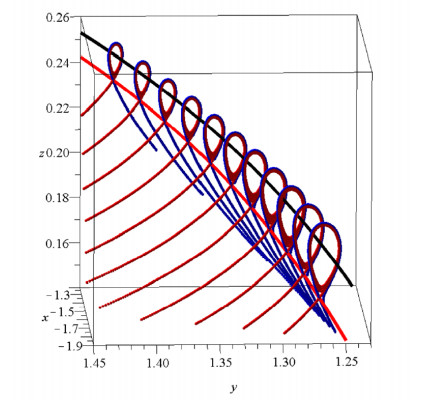
My own involvement in this problem started during my visit in Stockholm in 1958. At the suggestion of the leading Swedish Astronomer Prof. Bertil Lindblad. I extended his work of first order epicyclic orbits on the plane of a galaxy to all higher orders [19]. Then I tried to extend my calculations to the third dimension. Very little work existed at that time on the vertical oscillations. Thus I calculated on the computer BESK of the University of Stockholm two orbits on the meridian plane of a very simple model of the galactic Hamiltonian:
| $ H=12(˙x+˙y+ω21x2+ω22y2)+εxy2+ε′x3=h $ | (1.1) |
representing the motions of stars near the Sun.
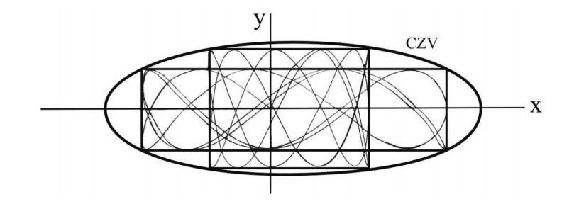
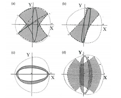
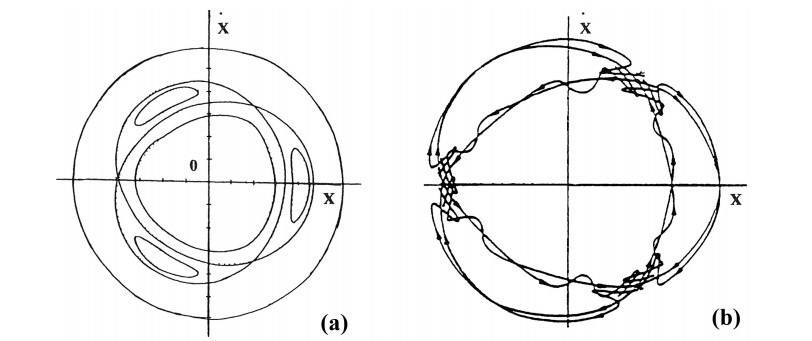
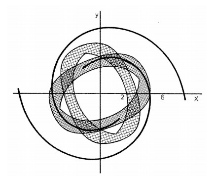
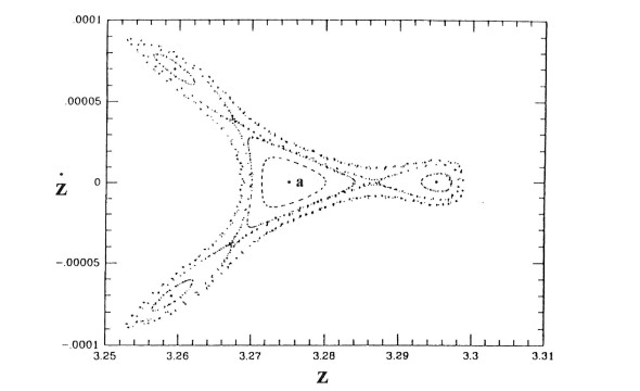
The results were surprising (Figure 1). I expected that the orbits should fill the whole space inside the Curve of Zero Velocity (CZV), but instead they filled two different "curvilinear parallelograms", in a way similar to Lissajous figures. I published these orbits in 1958 [20] and I presented my results at a special meeting of the IAU General Assembly in Moscow (1958). At the meeting there was Dr. G. Kuzmin, who commented that my calculations indicated the existence of a third integral in this galactic model. I replied that the existence of a third integral was not probable for two reasons: (a) the theoretical nonexistence theorems of Poincaré and Fermi and (b) because the system I considered was so simple that if there was a third integral someone would have found it already. In fact, later I realized that in fact Whittaker [126,127], Cherry [15,16,17] and Birkhoff [7] had found formal integrals in similar cases.
After the Moscow meeting Dr. Kuzmin wrote me on 7-2-59: "I think that the Poincaré theorem is applicable to the third integral problem and that it proves the non-existence of this integral in general case... Although these considerations are perhaps not fully free from gaps they dispel to a great extent my doubts about the non-existence of the one-valued third integral in general case...".
But meanwhile I could calculate a formal third integral in the form of a series and I presented my results at the Kiel meeting of the Deutsche Astronomische Gesellschaft in 1959. Thus I replied to Dr. Kuzmin on 29-9-59: "Meanwhile I have found a third integral in a special case, and then in a quite general case. I made a short communication about this problem in the Kiel Meeting of the Deutsche Astronomische Gesellschaft. I include herewith a short summary of this communication. I will send you a complete copy of my paper as soon as I have one available".
In fact my paper appeared in the Zeitschrift für Astrophysik in 1960 [21] and Dr. Kuzmin wrote me in 15-7-60: "Recently I found in ZAp your very interesting paper about which you spoke in your letter. Your paper inspired me to return to the problem at last".
The third integral of the Hamiltonian (1) is a series of the form:
| $ Φ=Φ2+Φ3+Φ4+... $ | (1.2) |
where
| $ Φ2=12(˙x2+ω12x2) $ | (1.3) |
is the energy along the x-axis (in the lowest order). The third order term is:
| $ Φ3=1(ω12−4ω22)[(ω12−2ω22)x1x22−2x1y22+2y1x2y2] $ | (1.4) |
and higher order terms can be calculated step by step.
At the Kiel meeting there was present Prof. Otto Heckmann who was very much interested in my work and encouraged me to proceed further. In particular he wanted me to prove the convergence of the third integral. However I could not find any such proof and I left the problem open.
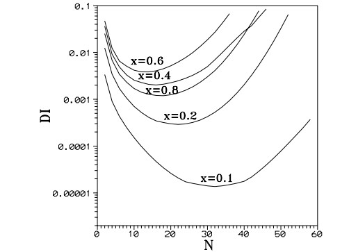
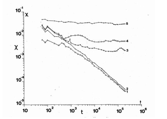
Later I realized that in general the third integral is not convergent, but only formal. In fact if we truncate the third integral at successively higher orders we find first a better and better convergence, but beyond a certain order the values of the truncated third integral have larger and larger deviations (Figure 2) [51]. As $ x $ increases the best truncation occurs at smaller orders. This is consistent with the Nekhoroshev [108] theorem for formal series.
Nevertheless formal series may give very useful approximate results. An example was provided by Poincaré [111] who considered the series.
| $ fi=∞∑n=0n!(1000)n $ | (1.5) |
This series is divergent, but if we truncate it at high orders smaller than $ n = 1000 $, we find very constant results. On the other hand the series
| $ fi=∞∑n=0(1000)nn! $ | (1.6) |
is convergent but requires orders higher than $ n = 1000 $ in order to show its convergent character.
Thus Poincaré states that while the mathematicians consider (correctly) the first series is divergent and the second convergent, the astronomers on the contrary consider the first series convergent and the second divergent, because their numerical calculations never go to very high orders.
One of the first astronomical applications of the third integral was in finding the forms of the velocity ellipsoid in our Galaxy. It was observed that the velocities of the stars near the Sun are distributed around the velocity of the Sun with decreasing densities outwards, the equidensities forming three-axial ellipsoids. If there were only two integrals of motion, the energy $ E = \frac{1}{2}(\dot{r}^2 + \Theta^2 + \dot{z}^2) + V(r, z) $ and the z-component of the angular momentum $ A = r \Theta $ one would expect a distribution function
| $ f(E,A) $ | (1.7) |
that would have the $ \dot{r} $ and $ \dot{z} $ axes equal. However the observed distribution gives the $ \dot{z} $-axis much smaller than the $ \dot{r} $-axis. This can be explained if a third integral $ \Phi = \frac{1}{2}\dot{z}^2 +... $ exists beyond the two other integrals. Then the $ r $ and $ z $ axes do not need to be equal. (This was the thesis of B. Barbanis [5]).
Much work on the third integral had been done by Whittaker [126,127] who called this integral "adelphic" (from the Greek word "adelphos" = brother) and also by Cherry [15,16,17] and Birkhoff [7]. Whittaker used action-angle variables while Cherry and Birkhoff used complex variables. My own work was using cartesian variables that are very useful for galactic applications. Furthermore I used a computer program to calculate higher order terms of the third integral, that gave very good approximate results ([24,43]).
Another important development around that time was the celebrated KAM theorem [1,2,3,92,105,106]. This theorem states that in an autonomous Hamiltonian system, close to an integrable system expressed in action-angle variables, there are N-dimensional invariant tori containing quasi-periodic motions with frequencies $ \omega_i $, satisfying a diophantine condition (after the ancient Greek mathematician Diophantos):
| $ |ωk|>γkN, $ | (1.8) |
where
| $ ωk=ω1k1+ω2k2+…ωNkN, $ | (1.9) |
with $ k_1, k_2, \dots, k_N $ integers and $ |k| = |k_1|+|k_2|+\dots |k_N|\neq 0 $, while $ \gamma $ is a small quantity depending on the perturbation. Thus if a system is close to integrable and the frequencies $ \omega_i $ are far from all resonances the orbits lie on invariant tori.
On a surface of section of a 2-D system these tori form invariant curves around a stable invariant point which is the intersection of a stable periodic orbit.
It is remarkable that Birkhoff [7] did not believe in the existence of such invariant curves and stated that orbits starting close to an invariant point of the stable type would gradually go very far from it.
The KAM theorem had many important applications in various dynamical systems. It was later supplemented by the Nekhoroshev theorem [108], that used expansions of the third integral type to approximate the motions in non-integrable systems close to an integrable system. Namely if the deviation from an integrable system is of order $ \varepsilon $, the formal integrals are valid over an exponentially long time of the order of
| $ t=t∗exp(Mετ), $ | (1.10) |
where $ t_*, M $ and $ \tau $ are positive constants. This time in particular astronomical problems may exceed the age of the universe.
Improvements of the Nekhorosev theory were provided by Giorgilli [77,78] and in particular by Morbidelli and Giorgilli [102] who found superexponential stability times. In the limiting cases of the KAM tori this time goes to infinity [81]. Therefore the KAM theorem is a limit of the Nekhorosev theorem. Further developments of the Nekhorosev theory were provided by Contopoulos, Efthymiopoulos and Giorgilli in [51] and by Efthymiopoulos, Giorgilli and Contopoulos in [68].
Around 1962 I had some interesting interactions with J. Moser. At first Moser did not believe that asymptotic series like that of the third integral were useful. But he asked me to give a seminar on this subject at the Courant Institute in New York in 1962. When he saw how well the third integral was conserved (I had at that time computer calculations up to the 10th order) he was impressed. Later he wrote in a paper [107] "These questions received renewed interest on account of the work of Contopoulos, who searched for and calculated a "third integral" for a system describing a galactic model".
When I was a visiting professor at the Yale University (1962) I gave a series of lectures on the third integral. I summarized my lectures in a paper [22] under the title "On the existence of a third integral of motion". I had included in this paper a section devoted to the use of a "surface of section" to visualize the orbits in the phase space of a conservative system of 2 degrees of freedom. My paper was accepted and I had received the proofs, when the referee sent me a belated remark, that the surface of section part of my paper was not so important and it would be good to omit it. Thus I took out this part. That was a mistake because soon afterwards there was the famous paper by Hénon and Heiles [87] under the title "The Applicability of the Third Integral of Motion: Some Numerical Experiments" that was based mainly on figures drawn by the computer on a surface of section.
During my stay at Yale I organized a meeting on dynamical systems that was attended by Moser, Hénon, Toomre, Szebehely, Brouwer etc. Moser spoke about the KAM theorem. But when I asked him if he could give an estimate of the applicability of his theorem to a practical problem like the Sun-Earth-Moon system, he refused to give such an estimate.
Then Hénon made some calculations in his hotel and next day he gave an estimate for the convergence of the KAM theorem that was published later [85]. This estimate was $ 10^{-48} $ in some appropriate units, which would imply that the orbit of the Moon would be stable despite the perturbation due to the Sun, if the Earth and the Moon were point masses at a distance less than 1mm. Later, however, it was shown that the KAM theorem was giving realistic results in many real cases. As a consequence people could apply the third integral to prove the stability of the Trojan asteroids at distances from the equilateral equilibria $ L_4 $ and $ L_5 $ of the order of 1 astronomical unit [64,67].
During my stay at Yale I had a Greek student, Mr. G. Bozis, and I suggested to him to study numerically the restricted three-body problem (RTBP) to find whether a third integral was applicable in this case. Then I left Yale. Bozis asked permission from his supervisor, Prof. V. Szebehely to use the computer to calculate orbits in the restricted problem. But Prof. Szebehely was reluctant. He told him that it was known that Poincaré's theorem is applicable in the RTBP, thus there should be no third integral in this case. Bozis, however insisted and finally Szebehely reluctantly agreed to let Bozis use the computer for these calculations, but he told him "You do that at your own risk". But when Bozis got his first results Szebehely was amazed. Bozis' figures indicated a well established third integral.
After my return to Greece (1964) I organized an IAU Symposium in Thessaloniki on "the theory of orbits", that was attended by many people working in Celestial Mechanics and Stellar Dynamics. Among them there were Hénon and Szebehely. Hénon spoke about the orbits in the restricted three-body problem and showed many figures indicating the existence of a third integral [86]. Then Szebehely jumped up at the discussion period saying that he had done similar work with G. Bozis, a student of Prof. Contopoulos. He presented many figures, making essentially a second lecture on the subject [118]. Bozis published his results in detail later [11].
The third integral was very useful in calculating the usual types of orbits in a Galaxy ("boxes", i.e., deformed Lissajous figures, like those in Figure 1 or more deformed as in Figure 3) The agreement between the theoretical results and the numerically calculated orbits was perfect. But Torgard and Ollongren [119] had found also "tube orbits" i.e., orbits filling tubes around various stable periodic orbits. While I was at Yale (1962) I found also several types of tube orbits (Figure 4) using the IBM 707 computer of the Institute of Space Sciences in New York.
At first people thought that the third integral was not applicable to such tube orbits. However at that time I developed the theory of the resonant forms of the third integral and I concluded that the tube orbits were due to particular resonances.
After my return to Greece (1963) I continued using the computers of the Institute of Space Studies by mail. I was sending the initial conditions of the orbits to a friend of mine at the Institute of Space Studies, in the form of punched cards. After about one month I was receiving the output, mainly in the form of figures, done by the computer. (Today such calculations are done in a few seconds).
Most orbits in the meridian plane of a galaxy were boxes. But I found that some initial conditions should lead to particular tube orbits. I sent these initial conditions to my friend in New York. When the results arrived, in the form of a thick roll of computer figures, the whole Astronomy Department was excited. We were looking with anxiety at the figures, as we developed the roll on the corridor. And behold! There appeared the nice tube orbits that we expected. And we saw also the expected transitions from the tube to the box orbits. These results were published later [23,25].
The calculation of the higher order terms of the third integral cannot be done by hand, as there are many thousands or millions of terms to be calculated. Thus I decided to write a computer program to calculate these higher order terms. At that time there were no packages of computer algebra, like Mathematica etc. Thus I wrote a program in Fortran that could calculate the third integral up to order 12. We had an IBM 1620 computer at the University of Thessaloniki, and we used punched cards. Because of limitations in memory I had to split my program in two parts. The first part produced a deck of cards 1 meter long. This was used as an initial condition for the second part, that produced a deck 2 meters long, and this finally was used to calculate our orbits, periodic orbits etc. The results were impressive. We published these results in 1965 [43] and in more detail in [24]. A little later Gustavson [82] prepared a similar paper, also finding higher order terms of the normal form (equivalent to the third integral).
When $ \omega_1 = \omega_2 $ the form of the third integral changes completely. It is not a part of the energy, as in non resonant cases. The forms of the orbits in this case are very different from distorted Lissajous figures (Figure 5) [25,43,44].
I was in Chicago in 1969 when I saw Dr. Chandrasekhar in the corridor carrying a gadget to show to his students. This contained a sphere that could go up and down, or rotate around its vertical axis. Chandrasekhar wanted to show the coupling between the up and down oscillation and the rotational oscillation. If one would set the sphere in the up and down mode, later this up and down motion would gradually stop and all the energy would go in a rotational oscillation clockwise and counterclockwise. Even later the rotation would stop and the energy would return to the up and down motion and so on.
The use of an "experiment" by Chandrasekhar was quite unusual. Then Chandra told me "You see, George, a case where your third integral is not applicable". But, as I explained to him, this was a perfect case of a 1:1 resonance, where the third integral has a very different form.
One important application of the resonant forms of the third integral is in finding periodic orbits. Poincaré has indicated that the periodic orbits are dense in generic dynamical systems, both integrable and nonintegrable.
A periodic orbit in an autonomous Hamiltonian
| $ H(x,y,˙x,˙y)=h $ | (2.1) |
has two characteristic exponents zero and a pair of exponents $ \pm \alpha $ opposite to each other. If there is another integral of motion
| $ Φ(x,y,˙x,˙y)=c $ | (2.2) |
then either $ \alpha = 0 $ or
| $ ΦxHx=ΦyHy=Φ˙xH˙x=Φ˙yH˙y $ | (2.3) |
(where $ \Phi_x = \partial{\Phi}/\partial{x} $ etc) which means that the surfaces $ H $ and $ \Phi $ are tangent along the periodic orbit. We found many cases where the latter relation is satisfied. However for every resonance the form $ \Phi $ of the third integral is different.
If we replace $ \dot{y} $ from Eq. (2.1) into Eq. (2.2) we have on a surface of section (say $ y = 0 $), for a given energy $ h $, an invariant curve
| $ F(x,˙x)=c $ | (2.4) |
The periodic orbits are singular points on this surface of section
| $ Fx=Fy=0 $ | (2.5) |
We found several resonant orbits in this way using our computer program to calculate the third integral [24]. In some cases we needed to use high order truncations in order to find periodic orbits with sufficient accuracy [27].
However in order to find the third integral up to very high order an effective computer program was necessary. This was done in a way that was quite unexpected. I was invited by two Italian Professors, Scotti and Galgani, to the Cagliari meeting of the Italian Physical Society (1972). I arrived an evening at Cagliari, and Scotti and Galgani were waiting for me at the airport. We went to my hotel and discussed many problems related to the third integral. The discussion continued the next day before and after the meeting of the Physical Society and then they drove me to the airport in the afternoon. I did not see Cagliari or Sardinia at all. But our discussion had one important consequence. When Galgani returned to Milan, he found a student (Giorgilli) who was eager to follow up this problem. And Giorgilli produced the best computer program to calculate the third integral to very high orders [76,80]. Giorgilli used a computer program that calculates the "generating function", the normal form and the integrals as series in the original variables. This method was a variant of the Lie series method of Hori [89] and Deprit [63].
The calculation of high orders was necessary because for low orders the third integral looked exact. E.g., Kaluza and Robnik [90] calculated the new integral in the Hénon-Heiles [87] problem up to order 14 and they found that the system looked integrable. Only if one goes at least to order 40 one sees definitely that the system is not integrable.
Later Efthymiopoulos calculated also high order integrals and applied them to the Trojan asteroids around the Lagrangian points $ L_4 $, $ L_5 $ of the solar system [64].
The periodic orbits for relatively small perturbations follow a regular pattern (Figure 6) for the Hamiltonian
| $ H≡12(˙x2+ω21x2+˙y2+ω22y2)−ϵxy2=h $ | (2.6) |
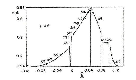
with $ \epsilon = 4.0 $ ($ \omega_1^2 = 1.6, \omega_2^2 = 0.9, h = 0.00765 $).
Every periodic and nonperiodic orbit has a particular rotation number and on the left the successive rotation numbers seem to vary smoothly in general. Only near $ 2/3 $ on the left of Figure 6 the decrease is abrupt (indicating chaos) and on the right there is an island of stability, where the rotation number is constant. In fact near every stable orbit there is a small plateau and the curve rot as a function of $ \overline{x} = \omega_1x $ is a "devil's staircase". In any case nonperiodic orbits form invariant curves with non rational rotation numbers and that set has a large measure. In fact the resonant effects around any rational $ n/m $ appear when the difference of the ratio $ \omega_1/\omega_2 $ from $ n/m < 1 $ is smaller than $ \varepsilon/m^3 $ i. e.,
| $ |ω1ω4−nm|<εm3 $ | (2.7) |
Therefore the resonant effects affect an interval $ 2\varepsilon/m^3 $. The sum of all the resonant intervals for $ n < m $ is smaller than
| $ ∞∑m=1m−1∑n=12εm3<2ε∞∑m=11m2=2εc, $ | (2.8) |
where $ c = 1.64 $ [38]. Thus if $ \varepsilon $ is small the total set of near resonant values of $ \omega_1/\omega_2 $ is small.
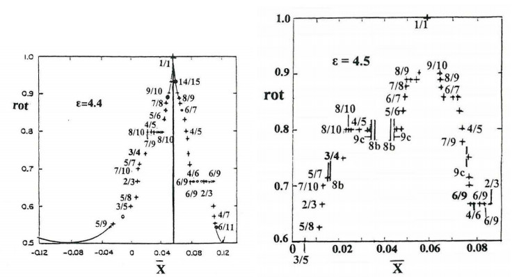
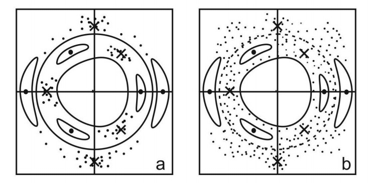
But when the perturbation increases (Figure 7a) to $ \varepsilon = 4.4 $ most invariant curves are destroyed. However the periodic orbits (mostly unstable) remain. Then for even higher perturbations (Figure 7b) $ \varepsilon = 4.5 $ a new type of periodic orbits appear, which are called "irregular" (vertical lines) [28]. These have in general rotation numbers different from those of their surroundings, or do not have any definite rotation number at all. In fact while most periodic orbits are produced as bifurcations of the central periodic orbit (1:1), or of the boundary, at smaller energies, the irregular orbits are produced in couples (one stable and one unstable) at a minimum $ \varepsilon $ (this is called a "tangent bifurcation"). The number of irregular orbits increases exponentially with their multiplicity $ m $, while the number of regular orbits increases as $ O (m^2) $ [50]. Thus the irregular orbits dominate the system for large perturbations.
Many irregular orbits are found in the lobes of the asymptotic curves of any unstable periodic orbit $ O $. The lobes are formed by the intersection of the stable and unstable manifolds (asymptotic curves) from the periodic orbit (Figure 8). Such orbits cannot be regular, i.e., they are not bifurcations of regular orbits that exist outside the loops. In fact, if there would be a continuous family of orbits inside and outside a loop there should be a case where the orbit would cross the boundary of the loop and this orbit would be asymptotic and not periodic. This was verified later by Simó and Vieiro [115].
The third integral is applicable if the perturbation of an integrable system is small. If the perturbation is large most orbits are chaotic and the third integral is destroyed.
Chaos appears in nonintegrable systems near the unstable periodic orbits. E.g., on a surface of section around an equilibrium point we may have a set of 3 islands around 3 points representing a stable periodic orbit and 3 chaotic regions around 3 points representing an unstable periodic orbit (Figure 9b).
In an integrable case there is no chaos and the 3 unstable points are joined by two separatrices (asymptotic curves forming the limits of the islands around the 3 stable points. (Figure 9a)). However if we calculate the asymptotic curves from the 3 unstable points in a nonintegrable case, they are intersected at an infinity of homoclinic points (Figure 9b). These intersections generate chaos, i.e., most nearby orbits form a set of scattered points on a surface of section (Figure 10) close to the unstable periodic orbits and their asymptotic curves.
In a nonintegrable system there is an infinity of stable and unstable periodic orbits at various distances from the equilibrium point. For small perturbations the islands of various orders and the chaotic regions around every unstable orbit are well separated by invariant (KAM) curves closing around the origin (Figure 10a). However when the perturbation increases the various resonances overlap (Figure 10b) and a large degree of chaos is generated. Then the KAM curves around the origin are destroyed and the third integral is no more applicable. \clearpage
A way to find the critical perturbation when large chaos is introduced and the third integral breaks down is by calculating the sizes of the islands using a different resonant form of the third integral for every set of islands. I did such a calculation in 1966 [26]. Around the same time a similar calculation was done by Rosenbluth et al. [113]. If the theoretical sizes of the islands become larger than the distance between the various types of islands it is obvious that the theoretical results are not valid any more and an overlap of resonances appears.
The theory of resonance overlap was later developed in detail by Chirikov [18] and by many authors it is called Chirikov's criterion. However Chirikov refers to my early paper [26] and to the paper of Rosenbluth et al. [113] when dealing with this problem [128]. I had sent my 1966 paper to Chirikov and he wrote me on 23-10-68: "My criterion of stochasticity by resonance overlapping is essentially the same as yours in your paper in Bulletin Astronomique".
A way to find whether an orbit is ordered or chaotic is by calculating its maximal Lyapunov characteristic number (LCN). Namely if $ \boldsymbol{\xi}, \boldsymbol{\xi_0} $ are the infinitesimal deviations from this orbit at times $ t $ and $ t_0 = 0 $ we have
| $ LCN=limt→∞χ=limt→∞ln|ξ/ξ0|t $ | (3.1) |
where $ \chi $ is the "finite time LCN". If $ LCN = 0 $ the orbit is ordered while if $ LCN > 0 $ the orbit is chaotic.
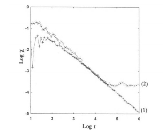
In numerical calculations we find that $ \log \chi $ has irregular variations for small t but as $ \log t $ increases it tends to vary linearly downwards for ordered orbits (orbit (1) in Figure 11, or it tends to a constant value (orbit (2) in Figure 11).
Theoretically $ \boldsymbol{\xi} $ was found by Contopoulos, Galgani and Giorgili [47] as a function of $ \boldsymbol{\xi_0} $ and $ t $ by solving the variational equations together with the equations of motion.
As the calculation of the limiting values of $ \chi $ requires a long computer time, there have been various more efficient methods for finding ordered and chaotic domains in dynamical systems. In particular in mappings one can use the "stretching number"
| $ an=ln|ξn+1/ξn| $ | (3.2) |
i.e., a local LCN, after only one iteration. Then after about 20 successive iterations we can find whether an orbit is ordered or chaotic [125]. Similar methods were developed by several other authors. A comparison of the various methods can be found in my book [38].
During my stay at the Yerkes Observatory in 1963 Dr. L. Woltjer visited us and we had many discussions about the third integral. Woltjer argued that my integral was applicable only to smooth potentials but could not be applied to more complicated cases, like the spiral arms of a galaxy. Dr. Chandrasekhar was present during our discussions and he sided with Woltjer. But the evening, during the dinner, I could convince Woltjer that I was right. The next morning Dr. Chandrasekhar told me "George, I thought about your problem and I think that Woltjer is right". But I replied "Chandra you are supposed to be an arbiter between me and Woltjer. But now Woltjer agrees with me. Thus you are obliged to agree also". Then Woltjer and I wrote a paper on a rough model of a spiral galaxy, that was published later [46]. This was a parallel approach to the density wave theory of spiral galaxies that was developed at that time by Lin and Shu [97].
The density wave theory of the spiral galaxies was first developed by Lindblad [98]. His work was most remarkable, since it predated the theory of plasma density waves. Lindblad pointed out, correctly, that this theory was applicable both to trailing and to leading spirals [99]. However Lindblad was prejudiced in favor of leading spirals [99], something that was objected by the majority of astronomers. This fact and the mathematical difficulties of his papers made most people to disregard his work.
When I met C. C. Lin in Boston, during my visit there in 1963, he told me that he wanted to develop a density wave theory of spiral structure. I told him that Lindblad had already done such a theory and we found in the MIT library several related volumes of the Stockholm Observatoriums Annaler. However the next day C. C. Lin told me that he found Lindblad's papers too difficult to follow, thus he would try to develop a theory from scratch ([97], and later papers).
Later I was involved quite a lot in the density wave theory. While Lin and Shu, and others, developed the linear theory, I developed a nonlinear theory [29,31] that is particularly useful near the resonances. In a galaxy we have two basic frequencies, the epicyclic frequency $ \omega_1 $ and the angular frequency $ \omega_2 $ in a frame rotating with the spiral arms. We have a resonance when $ \omega_1 / \omega_2 = m / n $ (integers). The linear theory is a first order theory away from resonances, but it is not applicable near the main resonances of a galaxy, the inner and outer Lindblad resonances, where $ \omega_1 / \omega_2 = \pm 2/1 $, and corotation (particle resonance), where $ \omega_2 = 0 $ [30].
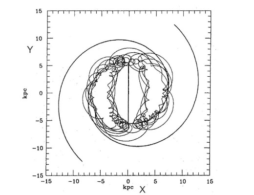
I could show that the nonlinear theory is an application of the third integral theory. In particular the third integral gives the main periodic orbits in the galaxy. Away from the resonances the spiral arms can be constructed by the successive periodic orbits, which are like precessing ellipses (Figure 12). The density maxima are along two symmetric spirals, where the successive orbits approach each other.
However near the inner Lindblad resonance there are two populations of near elliptical periodic orbits (Figure 13) perpendicular to each other. Outside this resonance the dominant family of periodic orbits forms the usual maxima along the spiral arms, while inside the resonance the response density is completely out of phase with the imposed density and tends to destroy it. Thus finally the density wave terminates near the inner Lindblad resonance.
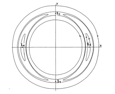
On the other hand near corotation we have two couples of families of periodic orbits, close to the Lagrangian points $ L_1 $, $ L_2 $ (unstable) and $ L_4 $, $ L_5 $ (stable unless there is a very strong bar at the center of the galaxy ($ L_3 $), in which case $ L_4 $, $ L_5 $ become unstable). Around the stable $ L_4 $, $ L_5 $ orbits there are vortices formed by banana-like orbits (Figure 14) [30].
A secondary but important resonance is the $ 4/1 $ resonance. Near this resonance the periodic orbits have the form of squares with smooth corners (Figure 12) [35]. However, while inside the resonance the orbits support the spiral arms (thick curves), outside the resonance the orbits have a quite different orientation and do not support the spirals. As a consequence the relatively strong spirals (of order $ 10\% $) must terminate near the $ 4/1 $ resonance, unless the amplitude of the spirals is quite small ($ < 5\% $), in which case weak extensions of the spirals can extend up to corotation.
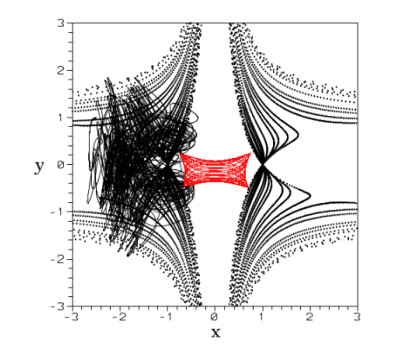
On the other hand in barred galaxies the perturbation is of order 50-100%. In such cases the orbits support the bar up to corotation, but tend to destroy it beyond corotation. Thus the bars terminate close but inside corotation [32]. (However there are cases where a bar terminates well inside corotation [120]). Beyond corotation we found that most orbits in barred galaxies are chaotic [91] (Figure 15).
The extension of our studies to 3 degrees of freedom opened new important areas of research. First of all we found new stability types of periodic orbits. In fact the eigenvalues (characteristic exponents) $ \lambda $ of a 3-d periodic orbit are given by an equation of the form
| $ λ4+aλ3+βλ2+aλ+1=0 $ | (5.1) |
The Eq. (5.1) can be factorized as follows:
| $ (λ2+b1λ+1)(λ2+b2λ+1)=0, $ | (5.2) |
where
| $ b1,2=12(a±√Δ) $ | (5.3) |
with
| $ Δ=a2−4(β−2) $ | (5.4) |
Thus the eigenvalues are
| $ λ1,2=12(−b1±√b21−4),λ3,4=12(−b2±√b22−4) $ | (5.5) |
(hence $ \lambda_1\lambda_2 = \lambda_3\lambda_4 = 1 $, i.e., the eigenvalues are inverse in pairs). If $ |b_1| < 2 $ and $ |b_2| < 2 $ the orbit is stable. Then the eigenvalues are complex conjugate on the unit circle. If $ |b_1| < 2, |b_2| > 2 $ the orbit is simply unstable. Then the eigenvalues $ \lambda_1, \lambda_2 $ are on the unit circle and the eigenvalues $ \lambda_3, \lambda_4 $ are on the real axis. Similarly if $ |b_1| > 2, |b_2| < 2 $. If $ \Delta > 0 $ and $ |b_1| > 2, |b_2| > 2 $ we have double instability and all eigenvalues are on the real axis. Finally if $ \Delta < 0 $ we have complex instability. Then the eigenvalues are complex of the form
| $ λ1,4=ea±iθ,λ3,2=e−a±iθ $ | (5.6) |
This classification is a simplification of a classification devised by Broucke [12].
E.g., in a Hamiltonian
| $ H≡12(˙x2+˙y2+˙z2+Ax2+By2+Cz2)−ϵxz2−ηyz2=h $ | (5.7) |
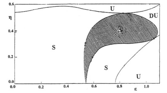
a particular type of periodic orbits (family 1a) in a diagram ($ \epsilon $, $ \eta $) has domains of stability (S), simple instability (U), double instability (UU) and complex instability ($ \Delta $)b (Figure 16)[42]. The most important type of instability is the complex instability ($ \Delta $ in Figure 16). (Details about the complex instability can be found in my book [38]). If we change the parameters A, B, C of Eq. (5.7) we can predict theoretically the behaviour of the various periodic orbits [34].
The periodic orbits can be found theoretically if we use the formal integrals of the "third integral" type.
If, besides the Hamiltonian (5.7) there is only one (formal) integral
| $ Φ(1)=Φ(1)(x,y,z,˙x,˙y,˙z)=c $ | (5.8) |
then a periodic orbit has either 4 characteristic exponents zero or
| $ Φ(1)xHx=Φ(1)yHy=Φ(1)zHz=Φ(1)˙xH˙x=Φ(1)˙yH˙y=Φ(1)˙zH˙z $ | (5.9) |
(the subscripts denote partial derivatives) This is similar to Eq. (2.3) in 2 dimensions. Then a family of periodic orbits depends on one parameter (the energy h).
If there are two (formal) integrals $ \Phi^{(1)} $ and $ \Phi^{(2)} $, then either all 6 characteristic exponents are zero or all the $ 3\times 3 $ determinants of the matrix
| $ \left( {HxHyHzH˙xH˙yH˙zΦ(1)xΦ(1)yΦ(1)zΦ(1)˙xΦ(1)˙yΦ(1)˙zΦ(2)xΦ(2)yΦ(2)zΦ(2)˙xΦ(2)˙yΦ(2)˙z} \right) $ | (5.10) |
are zero. Then a family of periodic orbits depends on 2 parameters.
If we solve Eq. (5.7) for $ \dot{z} $ and insert this value in Eq. (5.8) for $ z = 0 $ we find
| $ F=F(x,y,˙x,˙y,h)=c $ | (5.11) |
This represents a 3-D surface in the 4-D space $ (x, y, \dot{x}, \dot{y}) $. Then we have the following cases [33].
● Case 1. A periodic orbit is represented by a singular point. In this case the Eq. (5.9) are satisfied.
● Case 2. There is a family of periodic orbits for a given value of $ h $. Then Eqs. (5.9) are not satisfied and there are 4 characteristic exponents zero. But in this case the $ 3\times 3 $ determinants (5.10) are zero.
● Case 3. This is an exceptional case where all 6 characteristic exponents are zero.
Numerical experiments for the periodic orbits of the Hamiltonian (5.7) and other polynomial Hamiltonians have given good agreement with the theoretical calculations of periodic orbits using integrals $ \Phi^{(1)} $ and $ \Phi^{(2)} $ truncated at order 6.
I spoke about these new phenomena at a meeting in California (1985). After my talk I was approached by Prof. Lichtenberg, who told me "Usually the speakers at a meeting speak about a subject that they have covered, again and again, in previous meetings. Your talk was the only novel lecture today". After that we had long discussions with Profs. Lichtenberg and Lieberman at their Department. Later Lichtenberg and Lieberman [96] wrote a very interesting book on "Regular and Chaotic Dynamics", where they refer extensively to my work.
A numerical study of nonperiodic orbits in the system (5.7) [47] has shown a large ordered domain, an important chaotic sea, and smaller chaotic seas. In the ordered domain there are three formal integrals of motion, in the small seas there are two integrals and in the large sea there is only one integral (the energy).
Using the computer program of Giorgilli [79] we calculated 3 formal integrals
| $ Φi=Φi2+Φi3+…,(i=1,2,3) $ | (5.12) |
where $ \Phi_{in} $ contains terms of degree $ n $. In particular $ \Phi_{i0} $ are the harmonic energies along the axes x, y and z. We found that there is an ordered region where all these formal integrals (truncated at order 8) were approximately conserved, a large chaotic region (big sea) where all three formal integrals had large variations and only the total energy $ H = h $ was conserved, and some small regions (small seas) where we had one formal integral approximately conserved, besides the total energy.
A check of the validity of the integrals along particular orbits was made by calculating the finite time Lyapunov characteristic number $ \chi $ for a large interval of time. In the ordered region the value of $ \chi $ decreases linearly in time (Figure 17) thus the limiting value of $ \chi $ is zero. In the chaotic regions the value of the "finite time LCN" $ \chi $ tends to a constant $ LCN\neq 0 $. But in the big sea the limiting value of LCN is large (and independent of the initial conditions) while in every small sea the limiting LCN is maller than in the big sea. However the question is whether the small seas communicate with the big sea after a long time. This is probable because of Arnold diffusion (see below). If this happens then the final value of LCN for all chaotic orbits should be the same.
Arnold diffusion refers to a diffusion that appears in systems of three or more degrees of freedom despite the KAM theorem. In fact in a system of two degrees of freedom the KAM tori are 2-dimensional and separate the orbits in the 3-D phase space inside and outside these tori. However in a system of $ N\geq 3 $ degrees of freedom the KAM tori are N-dimensional in the 2N-1 phase space and do not separate an inner and an outer domain (E.g., if $ N = 3 $ the KAM tori are 3-dimensional in a 5 dimensional phase space). Thus there can be diffusion from one side of an invariant (KAM) torus to the other. This is called Arnold diffusion [4] and appears even if the perturbation from an integrable case is infinitesimal. Of course in an integrable case all orbits lie on invariant surfaces and no diffusion appears.
In order to understand the Arnold diffusion we may reduce all dimensions by 2. Thus the phase space is 3-dimensional and the KAM tori are 1-dimensional, like strings. These strings leave gaps around them and they allow the motions to go all over the 3-D phase space.
In the gaps between invariant tori there are resonant unstable periodic orbits surrounded by layers of chaotic orbits. These layers communicate with each other and generate Arnold diffusion.
The periodic orbits correspond to resonances of the form
| $ m1v1+m2v2+m3=0, $ | (5.13) |
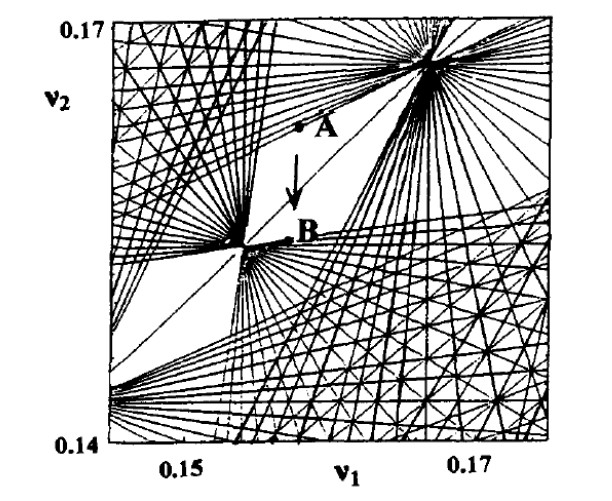
where $ v_1 = \omega_1/\omega_3, v_2 = \omega_2/\omega_3 $ and $ m_1, m_2, m_3 $ are integers. The lines in the plane $ (v_1, v_2) $ form the so called Arnold web (Figure 18). A chaotic orbit starting close to a point A can go close to a distant point B by following approximately successive lines of the web. Close to every intersection of these lines we have a resonances overlap and an orbit can go from one resonance to another.
The estimates for the diffusion rate according to Arnold are of order
| $ D∝exp(−1/√ε) $ | (5.14) |
where $ \varepsilon $ is the perturbation, therefore the diffusion is exponentially slow. However, if $ \varepsilon $ increases considerably the approximate lines become very thick and we may have a direct transition from A to B.
The phenomenon of Arnold diffusion was studied in detail by Froeschlé et al. [75] and other related works (see, e.g., [95]). A more extensive study was given recently by Efthymiopoulos and Harsoula [66] that shows clearly the details of Arnold diffusion.
Dr. Chandrasekhar and I had some rather interesting interactions on Relativity. Our first work was on the post-Newtonian approximations [14]. We first found the transformations of coordinates and time that generalize the Lorentz formulae in the first post-Newtonian approximation.
Later Chandrasekhar asked me to find order and chaos in the case of two fixed black holes. In fact Chandrasekhar [13] had calculated a few orbits in this case and he wanted me to distinguish between ordered and chaotic orbits. I wrote three papers on this topic [36,37,45] and this was the first systematic study of order and chaos in Relativity.
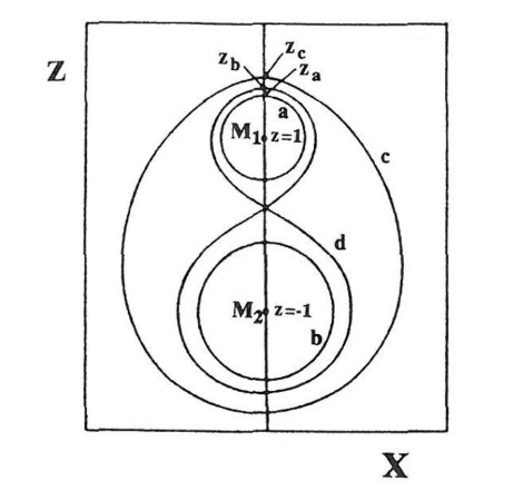
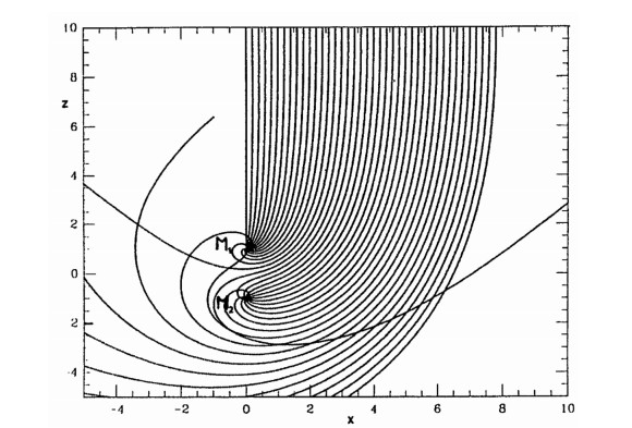
First of all I calculated the main periodic orbits around the two black holes (Figure 19) (orbits around the mass $ M_1 $ (a), or $ M_2 $ (b), and orbits surrounding both $ M_1 $ and $ M_2 $ (c), or forming a figure eight around $ M_1 $ and $ M_2 $ (d)). Then I distinguished orbits of type Ⅰ falling on $ M_1 $, of type Ⅱ falling on $ M_2 $ and of type Ⅲ escaping to infinity. There are infinite sets f orbits of type Ⅰ, Ⅱ and Ⅲ. In fact between 2 orbits of two different types (say Ⅰ and Ⅱ) there is an orbit of the third type (in this case Ⅲ) (Figure 20). (Between an orbit of type Ⅱ and an orbit of type Ⅲ there is an orbit of type Ⅰ and so on). Thus the orbits form fractal sets, and are in general chaotic. However there are some intervals of regular orbits. Namely there are some stable periodic orbits, surrounded by quasi-periodic orbits, as seen in Figure 21.
A by-product of this study was that in the classical problem of 2 fixed centers there are no periodic orbits of type (a) and (b) around a single mass $ M_1 $ or $ M_2 $. This fact had escaped the notice of previous authors on the two fixed centers, but I gave an analytic proof of the nonexistence of such orbits [36].
The case of relativistic order and chaos received much attention in the following years. In particular the question rose whether the mixmaster cosmological model is integrable or not. The mixmaster model [6,101] has expansion and contraction along different directions, which change in a chaotic way an infinite number of times as we approach the initial singularity (backwards in time), This problem can be written by the following Hamiltonian
| $ H≡12(p2x+p2y+p2z−2pxpy−2pypz−2pzpx)+e2x+e2y+e2z−2ex+y−2ey+z−2ez+x=0 $ | (6.1) |
with energy equal to zero. Then the question is whether this Hamiltonian has the Painlevé property [112], i.e., whether the solutions can be expressed in Laurent series of time around every singular point.
We found a general solution, depending on six arbitrary constants, which is of Painlevé type [48] and this provided an indication of integrability. However later it was realized [94], [49] that there is another general solution, which is not of Painlevé type. Thus the mixmaster model is not integrable.
But is the mixmaster model chaotic? In a paper by Cushman and Sniatycki [55] it is stated that the mixmaster model is not chaotic, while a paper by Cornish and Levin [54] states that the mixmaster model is chaotic.
I pointed out that both papers are correct from different points of view. The first paper proves that almost all mixmaster orbits escape to infinity, thus they cannot be ergodic. On the other hand the second paper emphasizes the fractal structure of the orbits. Thus although the mixmaster model is not chaotic in the usual sense (because its phase space is not finite) it is a case of "chaotic scattering".
I spoke about this problem in Moscow in 2000. Then a Russian participant (Dr. Cernin) presented a paper under the title "The Contopoulos' paradox". The paradox was my opinion that the above papers are both correct.
An important development in recent years was the study of order and chaos in quantum mechanics. In the Bohmian approach of quantum mechanics [57,58,59,60,61], [8,9] we can define orbits by using, besides the Schrödinger equation, the pilot wave equation.
| $ ˙¯r=ℏmℑ(∇ΨΨ), $ | (7.1) |
where $ \Psi $ is a solution of Schrödinger's equation and $ \Im $ indicates the imaginary part.
The Bohmian orbits are either ordered or chaotic (Figure 22). We found cases where the orbits are ordered classically and chaotic in the corresponding quantum problem, and vice versa, cases where the orbits are chaotic classically while the corresponding quantum orbits are ordered [65].
Then we checked whether the Born rule of quantum mechanics, that gives the probability as the square of the wavefunction
| $ P=|Ψ|2 $ | (7.2) |
can be derived theoretically. In fact Bohm and Vigier [10] claimed that an arbitrary initial particle distribution $ P $ tends asymptotically to $ |\Psi|^2 $.
However we found [65] that this is not the case for ordered orbits. On the other hand for chaotic orbits in most cases the value of $ P $ approaches $ |\Psi|^2 $, following an exponential law in time. This defines a quantum analog of the Nekhoroshev time of classical mechanics. However there are also exceptional cases where even some chaotic orbits do not follow the Born rule [52].
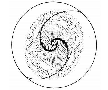
The solutions of Eq. (7.1) have a singular point when $ \Psi = \Psi_R+i\Psi_I = 0 $. This is called a nodal point. The orbits around the nodal point are of spiral form (Figure 23). The nodal point is either an attractor or a repellor. But close to the nodal point there is a second singular point (the X-point in Figure 23), which is unstable. If an orbit never approaches the region around the moving nodal point (the nodal point-X-point complex) then it is ordered and not chaotic (red orbit in Figure 22). However if an orbit approaches the region around the nodal point, then it is chaotic (black orbit in Figure 22).
The regular orbits can be given by series expansions involving trigonometric terms [69,40]. These series are similar to the classical formulae derived by the third integral theory for periodic time potentials. Chaos is generated when the orbits approach the X-point near the nodal point. This is an important new result in the dynamics of Bohmian quantum mechanics.
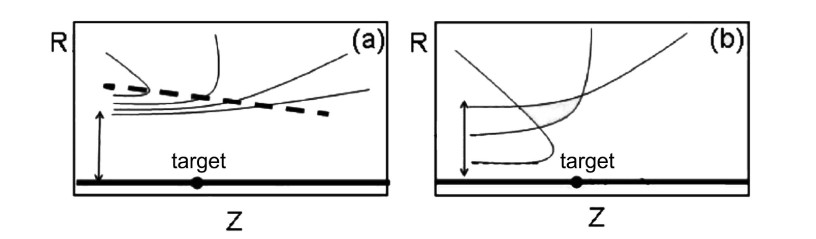
We considered also cases with more than one nodal point at every time [70] and cases of 3 dimensions [122,123]. Furthermore we found the diffraction patterns due to small material targets. In this case we have large numbers of nodal points along a line called "separator" (Figure 24)[62]. The particles follow nearly parallel orbits up to the separator, but their orbits deviate almost radially from the target beyond the separator. Orbits passing close to the target have small deviations, while orbits further away have larger deviations (Figure 24a). This behaviour is quite different from the classical picture (Figure 24b). where orbits coming close to the target have larger deviations than orbits passing further away.
The geometry of the quantum orbits explains the diffraction patterns observed in scattering experiments, including the appearance of enhanced flow along certain angles called Bragg angles.
An important consequence of this study is that the times of flight of orbits passing close to the target are larger than the times of flight of further away orbits (Figure 24a)[71]. This is the opposite of what happens in the classical case (Figure 24b) and requires an experimental verification that would support the Bohmian approach of quantum mechanics.
In 3 dimensions we have figures like Figure 23 at every level z. Thus we have nodal lines and X-lines (Figure 25). The orbits are chaotic if they approach these lines. In particular cases we have one or two integrals of motion. In the case of one integral (called partially integrable) the motions take place on a surface [53,121,122] (Figure 26) and can be either ordered (blue curve) or chaotic (red curve) on this surface. In the case of two integrals (integrable case) all orbits are ordered. However in general orbits have no integral, but are chaotic filling a volume in 3 dimensions (Figure 27).
An important recent development refers to the use of the third integral in calculating chaotic orbits. As it was shown by Moser [103,104] the third integral around an unstable periodic orbit is convergent. This is due to the fact that there are no small divisors in the series of the third integral in this case, while there are infinitely many small divisors in the series around a stable periodic orbit. In fact near a stable periodic orbit the (formal) integral has divisors of the form $ m_1\omega_1+m_2\omega_2 $ (where $ \omega_1 $ and $ \omega_2 $ are real and $ m_1, m_2 $ are integers) and some of these divisors are very small, generating nonintegrability. However near an unstable periodic orbit one eigenvalue is real and the other is imaginary, therefore the divisors $ m_1\omega_1+m_2\omega_2 $ never become small. This problem was first discussed by Cherry [17] and in more detail by Moser [103,104]. The proof of Moser was completed by Giorgilli [79]. The method of Moser was applied by da Silva Ritter et al. [56], Vieira and Ozorio de Almeida [124] and Ozorio de Almeida and Vieira [110] in finding the asymptotic curves and nearby orbits in the case of the Hénon hyperbolic map:
| $ x′=cosh(κ)x+sinh(κ)(y−x2√2)y′=sinh(κ)x+cosh(κ)(y−x2√2) $ | (8.1) |
Da Silva Ritter, Ozorio de Almeida and Douady [56] introduced a new, near to the identity transformation in the variables
| $ u=(x+y√2)=ξ+Φ12+Φ13+…v=(x−y√2)=η+Φ22+Φ23+… $ | (8.2) |
such that in the new variables ($ \xi, \eta $) the transformation becomes
| $ ξ′=Λ(c)ξ,η′=1Λ(c)η $ | (8.3) |
where
| $ c=ξη=ξ′η′=const $ | (8.4) |
and
| $ Λ=λ1+w2c+w3c2+... $ | (8.5) |
($ \lambda_1 $ being the largest eigenvalue of the mapping for a given $ \kappa $ and $ w_i $ are constants).
We extended this work by calculating the limits of applicability of the Moser series [72]. Namely the mapping (8.1) gives the consequents of an initial point $ (\xi_0, \eta_0) $ along a hyperbola $ \xi_0 \eta_0 = c $ (Figure 28a). The limiting value of $ c $ is found by using the d' Alembert criterion. Namely we calculated the limits of the ratios
| $ |Φi,n||Φi,n+1| $ | (8.6) |
along any given direction $ \phi $, where $ \xi = R \cos \phi, \, \eta = R \sin \phi $.
We found numerically that in this particular case the limits of the ratio (43) depend on $ R $ but not on $ \phi $.
For $ \kappa = 1.43 $ the series converge for $ |c| \leq 0.49 $ [83].
Any orbit with initial conditions inside the domain of convergence, has its images and pre-images along a hyperbola passing through this point (Figure 28a).
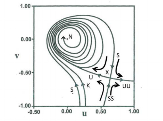
If we back-transform the hyperbolae of Figure 28a to the original variables $ (x, y) $, by inverting Eqs. (8.2), we find the image of the domain of convergence of the Moser series in the plane $ (x, y) $ (red in Figure 28b). This domain is limited outwards by the images of the curves $ c = \pm 0.49 $ of the regions 2, 3, 4 of Figure 28a. However there is also an inner limit, which is the image of the curve $ c = 0.49 $ of the region 1, in the ($ \xi, \eta $) plane. Thus there is an inner region (white in Figure 28b) where the series do not converge. This region is around a stable periodic point $ S $.
In Figure 29 we have drawn a number of invariant curves $ \xi \eta = c $ as they are mapped in the variables $ (x, y) $. We call these curves "Moser invariant curves". In particular the curves $ c = 0 $ (red) represent the axes $ \eta = 0 $ and $ \xi = 0 $. These curves correspond to the stable and unstable asymptotic curves of the point $ (0, 0) $ and extend to infinity within the domain of convergence, because the series (39) converge all the way to infinity if $ \eta = 0 $ or $ \xi = 0 $. The images of the curves $ \xi = 0 $ and $ \eta = 0 $ intersect each other at an unlimited number of homoclinic points that can be found analytically.
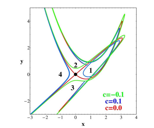
Any point in the domain of convergence (red) of Figure 28b has its images inside the same domain. On the other hand orbits with initial conditions outside the domain of convergence have images that approach closer and closer the outer limits of this domain. This is seen in Figure 28b where we have mapped a grid of initial conditions $ (-10, 10) \times (-10, 10) $ outside the convergence domain. Their first images are in green and their second images are in blue (covering also the inner green regions). Higher order images are congested even closer to the outer limits of the domain of convergence. Thus the outer limits of the domain of convergence acts as an attractor for the orbits outside this domain [41].
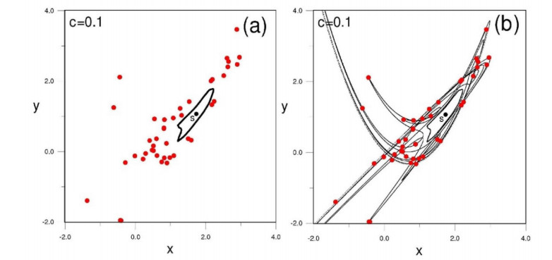
The main application of the Moser series regards the orbits starting close to the origin $ O $ where chaos is dominant. In this case the successive images of an initial condition close to $ O $ look quite random (Figure 30a). However, all these points lie on a particular Moser invariant curve (Figure 30b) that can be given accurately analytically. Thus these chaotic orbits can be given by analytical formulae. The only indication of chaos is that although all the iterates lie on the same Moser curve, the distance between successive iterates increases at every iteration. Furthermore, the Moser invariant curves make many oscillations that extend to large distances, therefore some points on them may be at considerable distances from the center.
A particular application of the Moser series is in finding periodic orbits.
In Figure 31 we give the characteristics of the various families 6, 5, 4, 3, 2 together with the characteristics of the periodic orbit $ S $ and of the homoclinic point $ H $. In particular the two families of period 4 are generated from the stable family $ S $ at $ \kappa = 1.317 $. The upper family is initially stable while the lower one is unstable. The stable family becomes unstable at a period doubling bifurcation, and all the families that were produced by a cascade of further bifurcations become unstable beyond $ \kappa = 1.383 $. The same happens with all the families of order higher than 4. All these families are congested close to the homoclinic point $ H $ for larger values of $ \kappa $ (Figure 31).
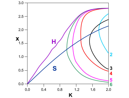
Of special interest is the family of period 2 because when this family is bifurcated from the original family $ S $ (for $ \kappa = 1.76 $), the orbit $ S $ itself becomes unstable. The bifurcating stable family 2 also becomes unstable at $ \kappa = 1.84 $ and then follows a cascade of periodic doubling bifurcations so that beyond $ \kappa = 1.86 $ all the bifurcated families become unstable.
When $ S $ becomes unstable it has its own asymptotic curves and new Moser invariant curves close to them. We found a Moser transformation that gives these new asymptotic invariant curves [41]. There is a Moser domain of convergence of these transformations (green) which is completely inside the Moser domain of convergence around the origin point $ O $ (red in Figure 32a). In this case ($ \kappa = 2 $) there is no inner limit of the domain of convergence around $ S $.
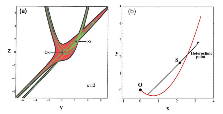
The asymptotic curves from the orbit $ S $ intersect the asymptotic curves from the orbit $ O $ at heteroclinic points (Figure 32b). All the homoclinic and heteroclinic points are found analytically with a very good accuracy as compared with the numerical results [41].
An application of the Moser series is in finding the chaotic orbits that generate the spiral arms outside corotation in barred galaxies [84]. In fact the spiral arms in barred galaxies are composed of chaotic orbits that can be given theoretically by using the Moser theory. Thus the use of the Moser series has important applications in galactic dynamics.
Further details about the history of the third integral can be found in the books of Contopoulos [38,39].
The author declares no conflict of interest.
| [1] | Leiman PG, Shneider MM (2012) Contractile tail machines of bacteriophages. In: Rossmann MG, Rao VB, editors. Viral Molecular Machines. New York Dordrecht Heidelberg London: Springer. 93-114. |
| [2] |
Michel-Briand Y, Baysse C (2002) The pyocins of Pseudomonas aeruginosa. Biochimie 84: 499-510. doi: 10.1016/S0300-9084(02)01422-0

|
| [3] |
Sarris PF, Ladoukakis ED, Panopoulos NJ, et al. (2014) A phage tail-derived element with wide distribution among both prokaryotic domains: a comparative genomic and phylogenetic study. Genome Biol Evol 6: 1739-1747. doi: 10.1093/gbe/evu136
|
| [4] |
Amos LA, Klug A (1975) Three-dimensional image reconstructions of the contractile tail of T4 bacteriophage. J Mol Biol 99: 51-64. doi: 10.1016/S0022-2836(75)80158-6
|
| [5] |
Leiman PG, Chipman PR, Kostyuchenko VA, et al. (2004) Three-dimensional rearrangement of proteins in the tail of bacteriophage T4 on infection of its host. Cell 118: 419-429. doi: 10.1016/j.cell.2004.07.022
|
| [6] |
Kostyuchenko VA, Chipman PR, Leiman PG, et al. (2005) The tail structure of bacteriophage T4 and its mechanism of contraction. Nat Struct Mol Biol 12: 810-813. doi: 10.1038/nsmb975
|
| [7] |
Effantin G, Hamasaki R, Kawasaki T, et al. (2013) Cryo-electron microscopy three-dimensional structure of the jumbo phage PhiRSL1 infecting the phytopathogen Ralstonia solanacearum. Structure 21: 298-305. doi: 10.1016/j.str.2012.12.017
|
| [8] |
Fokine A, Battisti AJ, Bowman VD, et al. (2007) Cryo-EM study of the Pseudomonas bacteriophage phiKZ. Structure 15: 1099-1104. doi: 10.1016/j.str.2007.07.008
|
| [9] |
Aksyuk AA, Kurochkina LP, Fokine A, et al. (2011) Structural conservation of the myoviridae phage tail sheath protein fold. Structure 19: 1885-1894. doi: 10.1016/j.str.2011.09.012
|
| [10] |
Schwarzer D, Buettner FF, Browning C, et al. (2012) A multivalent adsorption apparatus explains the broad host range of phage phi92: a comprehensive genomic and structural analysis. J Virol 86: 10384-10398. doi: 10.1128/JVI.00801-12
|
| [11] | Ge P, Scholl D, Leiman PG, et al. (2015) Atomic structures of a bactericidal contractile nanotube in its pre- and postcontraction states. Nat Struct Mol Biol. |
| [12] |
Basler M, Pilhofer M, Henderson GP, et al. (2012) Type VI secretion requires a dynamic contractile phage tail-like structure. Nature 483: 182-186. doi: 10.1038/nature10846
|
| [13] |
Kube S, Kapitein N, Zimniak T, et al. (2014) Structure of the VipA/B type VI secretion complex suggests a contraction-state-specific recycling mechanism. Cell Rep 8: 20-30. doi: 10.1016/j.celrep.2014.05.034
|
| [14] |
Clemens DL, Ge P, Lee BY, et al. (2015) Atomic structure of T6SS reveals interlaced array essential to function. Cell 160: 940-951. doi: 10.1016/j.cell.2015.02.005
|
| [15] |
Kudryashev M, Wang RY, Brackmann M, et al. (2015) Structure of the type VI secretion system contractile sheath. Cell 160: 952-962. doi: 10.1016/j.cell.2015.01.037
|
| [16] |
Heymann JB, Bartho JD, Rybakova D, et al. (2013) Three-dimensional structure of the toxin-delivery particle antifeeding prophage of Serratia entomophila. J Biol Chem 288: 25276-25284. doi: 10.1074/jbc.M113.456145
|
| [17] |
Shikuma NJ, Pilhofer M, Weiss GL, et al. (2014) Marine tubeworm metamorphosis induced by arrays of bacterial phage tail-like structures. Science 343: 529-533. doi: 10.1126/science.1246794
|
| [18] |
Veesler D, Cambillau C (2011) A common evolutionary origin for tailed-bacteriophage functional modules and bacterial machineries. Microbiol Mol Biol Rev 75: 423-433. doi: 10.1128/MMBR.00014-11
|
| [19] |
Leiman PG, Arisaka F, van Raaij MJ, et al. (2010) Morphogenesis of the T4 tail and tail fibers. Virology 7: 355. doi: 10.1186/1743-422X-7-355
|
| [20] |
Silverman JM, Brunet YR, Cascales E, et al. (2012) Structure and regulation of the type VI secretion system. Annu Rev Microbiol 66: 453-472. doi: 10.1146/annurev-micro-121809-151619
|
| [21] |
Ho BT, Dong TG, Mekalanos JJ (2014) A view to a kill: the bacterial type VI secretion system. Cell Host Microbe 15: 9-21. doi: 10.1016/j.chom.2013.11.008
|
| [22] |
Zoued A, Brunet YR, Durand E, et al. (2014) Architecture and assembly of the Type VI secretion system. Biochim Biophys Acta Mol Cell Res 1843: 1664-1673. doi: 10.1016/j.bbamcr.2014.03.018
|
| [23] |
Nakayama K, Takashima K, Ishihara H, et al. (2000) The R-type pyocin of Pseudomonas aeruginosa is related to P2 phage, and the F-type is related to lambda phage. Mol Microbiol 38: 213-231. doi: 10.1046/j.1365-2958.2000.02135.x
|
| [24] |
Liu Y, Schmidt B, Maskell DL (2010) MSAProbs: multiple sequence alignment based on pair hidden Markov models and partition function posterior probabilities. Bioinformatics 26: 1958-1964. doi: 10.1093/bioinformatics/btq338
|
| [25] | Felsenstein J (1989) Phylip: phylogeny inference package (version 3.2). Cladistics 5: 164-166. |
| [26] | Ackermann HW (2006) Classification of bacteriophages. In: Calendar R, editor. The Bacteriophages. New York, USA: Oxford University Press. 8-16. |
| [27] | Orlova EV (2012) Bacteriophages and their structural organisation. Bacteriophages 3-30. |
| [28] |
Ruska H (1942) Morphologische Befunde bei der bakteriophagen Lyse. Arch Gesamte Virusforsch 2: 345-387. doi: 10.1007/BF01249917
|
| [29] |
Ackermann HW (2011) The first phage electron micrographs. Bacteriophage 1: 225-227. doi: 10.4161/bact.1.4.17280
|
| [30] |
De Rosier DJ, Klug A (1968) Reconstruction of three dimensional structures from electron micrographs. Nature 217: 130-134. doi: 10.1038/217130a0
|
| [31] | Jacob F (1954) Induced biosynthesis and mode of action of a pyocine, antibiotic produced by Pseudomonas aeruginosa. Annales de l'Institut Pasteur 86: 149-160. |
| [32] |
Takeya K, Mlnamishima Y, Amako K, et al. (1967) A small rod-shaped pyocin. Virology 31: 166-168. doi: 10.1016/0042-6822(67)90021-9
|
| [33] |
Ishii SI, Nishi Y, Egami F (1965) The fine structure of a pyocin. J Mol Biol 13: 428-431. doi: 10.1016/S0022-2836(65)80107-3
|
| [34] | Shinomiya T, Shiga S, Kageyama M (1983) Genetic determinant of pyocin R2 in Pseudomonas aeruginosa PAO. I. Localization of the pyocin R2 gene cluster between the trpCD and trpE genes. Mol Gen Genet 189: 375-381. |
| [35] | Birmingham VA, Pattee PA (1981) Genetic transformation in Staphylococcus aureus: isolation and characterization of a competence-conferring factor from bacteriophage 80 alpha lysates. J Bacteriol 148: 301-307. |
| [36] |
Coetzee HL, de Klerk HC, Coetzee JN, et al. (1968) Bacteriophage-tail-like Particles Associated with Intra-species Killing of Proteus vulgaris. J Gen Virol 2: 29-36. doi: 10.1099/0022-1317-2-1-29
|
| [37] |
Gebhart D, Williams SR, Bishop-Lilly KA, et al. (2012) Novel high-molecular-weight, R-type bacteriocins of Clostridium difficile. J Bacteriol 194: 6240-6247. doi: 10.1128/JB.01272-12
|
| [38] | Matsui H, Sano Y, Ishihara H, et al. (1993) Regulation of pyocin genes in Pseudomonas aeruginosa by positive (prtN) and negative (prtR) regulatory genes. J Bacteriol 175: 1257-1263. |
| [39] |
Scholl D, Cooley M, Williams SR, et al. (2009) An engineered R-type pyocin is a highly specific and sensitive bactericidal agent for the food-borne pathogen Escherichia coli O157:H7. Antimicrob Agents Chemother 53: 3074-3080. doi: 10.1128/AAC.01660-08
|
| [40] |
Williams SR, Gebhart D, Martin DW, et al. (2008) Retargeting R-type pyocins to generate novel bactericidal protein complexes. Appl Environ Microbiol 74: 3868-3876. doi: 10.1128/AEM.00141-08
|
| [41] | Uratani Y, Hoshino T (1984) Pyocin R1 inhibits active transport inPseudomonas aeruginosa and depolarizes membrane potential. J Bacteriol 157: 632-636. |
| [42] |
Strauch E, Kaspar H, Schaudinn C, et al. (2001) Characterization of Enterocoliticin, a Phage Tail-Like Bacteriocin, and Its Effect on Pathogenic Yersinia enterocolitica Strains. Appl Environ Microbiol 67: 5634-5642. doi: 10.1128/AEM.67.12.5634-5642.2001
|
| [43] |
Ito S, Kageyama M, Egami F (1970) Isolation and characterization of pyocins from several strains of Pseudomonas aeruginosa. J Gen Appl Microbiol 16: 205-214. doi: 10.2323/jgam.16.3_205
|
| [44] |
Rodou A, Ankrah DO, Stathopoulos C (2010) Toxins and secretion systems of Photorhabdus luminescens. Toxins 2: 1250-1264. doi: 10.3390/toxins2061250
|
| [45] |
Yang G, Dowling AJ, Gerike U, et al. (2006) Photorhabdus virulence cassettes confer injectable insecticidal activity against the wax moth. J Bacteriol 188: 2254-2261. doi: 10.1128/JB.188.6.2254-2261.2006
|
| [46] |
Hurst MRH, Beard SS, Jackson TA, et al. (2007) Isolation and characterization of the Serratia entomophila antifeeding prophage. FEMS Microbiol Lett 270: 42-48. doi: 10.1111/j.1574-6968.2007.00645.x
|
| [47] |
Rybakova D, Radjainia M, Turner A, et al. (2013) Role of antifeeding prophage (Afp) protein Afp16 in terminating the length of the Afp tailocin and stabilizing its sheath. Mol Microbiol 89: 702-714. doi: 10.1111/mmi.12305
|
| [48] | Rybakova D, Schramm P, Mitra AK, et al. (2015) Afp14 is involved in regulating the length of Anti-feeding prophage (Afp). Mol Microbiol. |
| [49] | Ogata S, Suenaga H, Hayashida S (1982) Pock Formation of Streptomycetes endus with Production of Phage Taillike Particles. Appl Environ Microbiol 43: 1182-1187. |
| [50] |
Mougous JD, Cuff ME, Raunser S, et al. (2006) A virulence locus of Pseudomonas aeruginosa encodes a protein secretion apparatus. Science 312: 1526-1530. doi: 10.1126/science.1128393
|
| [51] |
Pukatzki S, Ma AT, Sturtevant D, et al. (2006) Identification of a conserved bacterial protein secretion system in Vibrio cholerae using the Dictyostelium host model system. Proc Natl Acad Sci USA 103: 1528-1533. doi: 10.1073/pnas.0510322103
|
| [52] |
Bingle LE, Bailey CM, Pallen MJ (2008) Type VI secretion: a beginner's guide. Curr Opin Microbiol 11: 3-8. doi: 10.1016/j.mib.2008.01.006
|
| [53] |
Boyer F, Fichant G, Berthod J, et al. (2009) Dissecting the bacterial type VI secretion system by a genome wide in silico analysis: what can be learned from available microbial genomic resources? BMC Genomics 10: 104. doi: 10.1186/1471-2164-10-104
|
| [54] | Bröms JE, Sjöstedt A, Lavander M (2010) The Role of the Francisella tularensis Pathogenicity Island in Type VI Secretion, Intracellular Survival, and Modulation of Host Cell Signaling. Front Microbiol 1: 136-136. |
| [55] | de Bruin OM, Duplantis BN, Ludu JS, et al. (2011) The biochemical properties of the Francisella Pathogenicity Island (FPI)-encoded proteins, IglA, IglB, IglC, PdpB and DotU, suggest roles in type VI secretion. Microbiology. |
| [56] |
Russell AB, Wexler AG, Harding BN, et al. (2014) A type VI secretion-related pathway in Bacteroidetes mediates interbacterial antagonism. Cell Host Microbe 16: 227-236. doi: 10.1016/j.chom.2014.07.007
|
| [57] |
Shalom G, Shaw JG, Thomas MS (2007) In vivo expression technology identifies a type VI secretion system locus in Burkholderia pseudomallei that is induced upon invasion of macrophages. Microbiology 153: 2689-2699. doi: 10.1099/mic.0.2007/006585-0
|
| [58] |
Leiman PG, Basler M, Ramagopal UA, et al. (2009) Type VI secretion apparatus and phage tail-associated protein complexes share a common evolutionary origin. Proc Natl Acad Sci USA 106: 4154-4159. doi: 10.1073/pnas.0813360106
|
| [59] |
Pell LG, Kanelis V, Donaldson LW, et al. (2009) The phage lambda major tail protein structure reveals a common evolution for long-tailed phages and the type VI bacterial secretion system. Proc Natl Acad Sci USA 106: 4160-4165. doi: 10.1073/pnas.0900044106
|
| [60] |
Lossi NS, Dajani R, Freemont P, et al. (2011) Structure-function analysis of HsiF, a gp25-like component of the type VI secretion system, in Pseudomonas aeruginosa. Microbiology 157: 3292-3305. doi: 10.1099/mic.0.051987-0
|
| [61] |
Bonemann G, Pietrosiuk A, Diemand A, et al. (2009) Remodelling of VipA/VipB tubules by ClpV-mediated threading is crucial for type VI protein secretion. EMBO J 28: 315-325. doi: 10.1038/emboj.2008.269
|
| [62] |
Lossi NS, Manoli E, Forster A, et al. (2013) The HsiB1C1 (TssB-TssC) complex of the Pseudomonas aeruginosa type VI secretion system forms a bacteriophage tail sheathlike structure. J Biol Chem 288: 7536-7548. doi: 10.1074/jbc.M112.439273
|
| [63] |
Zheng J, Ho B, Mekalanos JJ (2011) Genetic analysis of anti-amoebae and anti-bacterial activities of the type VI secretion system in Vibrio cholerae. PLoS One 6: e23876-e23876. doi: 10.1371/journal.pone.0023876
|
| [64] |
Zoued A, Durand E, Bebeacua C, et al. (2013) TssK is a trimeric cytoplasmic protein interacting with components of both phage-like and membrane anchoring complexes of the type VI secretion system. J Biol Chem 288: 27031-27041. doi: 10.1074/jbc.M113.499772
|
| [65] |
Durand E, Zoued A, Spinelli S, et al. (2012) Structural characterization and oligomerization of the TssL protein, a component shared by bacterial type VI and type IVb secretion systems. J Biol Chem 287: 14157-14168. doi: 10.1074/jbc.M111.338731
|
| [66] |
Robb CS, Nano FE, Boraston AB (2012) The structure of the conserved type six secretion protein TssL (DotU) from Francisella novicida. J Mol Biol 419: 277-283. doi: 10.1016/j.jmb.2012.04.003
|
| [67] |
Ma LS, Lin JS, Lai EM (2009) An IcmF family protein, ImpLM, is an integral inner membrane protein interacting with ImpKL, and its walker a motif is required for type VI secretion system-mediated Hcp secretion in Agrobacterium tumefaciens. J Bacteriol 191: 4316-4329. doi: 10.1128/JB.00029-09
|
| [68] | Das S, Chaudhuri K (2003) Identification of a unique IAHP (IcmF associated homologous proteins) cluster in Vibrio cholerae and other proteobacteria through in silico analysis. In Silico Biol 3: 287-300. |
| [69] |
Felisberto-Rodrigues C, Durand E, Aschtgen MS, et al. (2011) Towards a Structural Comprehension of Bacterial Type VI Secretion Systems: Characterization of the TssJ-TssM Complex of an Escherichia coli Pathovar. PLoS Pathog 7: e1002386. doi: 10.1371/journal.ppat.1002386
|
| [70] |
Rao VA, Shepherd SM, English G, et al. (2011) The structure of Serratia marcescens Lip, a membrane-bound component of the type VI secretion system. Acta Crystallogr D Biol Crystallogr 67: 1065-1072. doi: 10.1107/S0907444911046300
|
| [71] |
Miyata ST, Bachmann V, Pukatzki S (2013) Type VI secretion system regulation as a consequence of evolutionary pressure. J Med Microbiol 62: 663-676. doi: 10.1099/jmm.0.053983-0
|
| [72] |
Bernard CS, Brunet YR, Gavioli M, et al. (2011) Regulation of type VI secretion gene clusters by sigma54 and cognate enhancer binding proteins and cognate enhancer binding proteins. Journal of bacteriology 193: 2158-2167. doi: 10.1128/JB.00029-11
|
| [73] |
Kitaoka M, Miyata ST, Brooks TM, et al. (2011) VasH is a transcriptional regulator of the type VI secretion system functional in endemic and pandemicVibrio cholerae. J Bacteriology 193: 6471-6482. doi: 10.1128/JB.05414-11
|
| [74] |
Dong TG, Mekalanos JJ (2012) Characterization of the RpoN regulon reveals differential regulation of T6SS and new flagellar operons in Vibrio cholerae O37 strain V52. Nucleic acids research 40: 7766-7775. doi: 10.1093/nar/gks567
|
| [75] |
Basler M, Ho BT, Mekalanos JJ (2013) Tit-for-tat: type VI secretion system counterattack during bacterial cell-cell interactions. Cell 152: 884-894. doi: 10.1016/j.cell.2013.01.042
|
| [76] |
Basler M, Mekalanos JJ (2012) Type 6 secretion dynamics within and between bacterial cells. Science 337: 815. doi: 10.1126/science.1222901
|
| [77] |
Ho BT, Basler M, Mekalanos JJ (2013) Type 6 secretion system-mediated immunity to type 4 secretion system-mediated gene transfer. Science 342: 250-253. doi: 10.1126/science.1243745
|
| [78] |
Fritsch MJ, Trunk K, Diniz JA, et al. (2013) Proteomic Identification of Novel Secreted Antibacterial Toxins of the Serratia marcescens Type VI Secretion System. Mol Cell Proteomics 12: 2735-2749. doi: 10.1074/mcp.M113.030502
|
| [79] |
Mougous JD, Gifford CA, Ramsdell TL, et al. (2007) Threonine phosphorylation post-translationally regulates protein secretion in Pseudomonas aeruginosa. Nat Cell Biol 9: 797-803. doi: 10.1038/ncb1605
|
| [80] |
Kapitein N, Bonemann G, Pietrosiuk A, et al. (2013) ClpV recycles VipA/VipB tubules and prevents non-productive tubule formation to ensure efficient type VI protein secretion. Mol Microbiol 87: 1013-1028. doi: 10.1111/mmi.12147
|
| [81] |
Hsu F, Schwarz S, Mougous JD (2009) TagR promotes PpkA-catalysed type VI secretion activation in Pseudomonas aeruginosa. Mol Microbiol 72: 1111-1125. doi: 10.1111/j.1365-2958.2009.06701.x
|
| [82] |
Silverman JM, Austin LS, Hsu F, et al. (2011) Separate inputs modulate phosphorylation-dependent and -independent type VI secretion activation. Mol Microbiol 82: 1277-1290. doi: 10.1111/j.1365-2958.2011.07889.x
|
| [83] |
Casabona MG, Silverman JM, Sall KM, et al. (2013) An ABC transporter and an outer membrane lipoprotein participate in posttranslational activation of type VI secretion in Pseudomonas aeruginosa. Environ Microbiol 15: 471-486. doi: 10.1111/j.1462-2920.2012.02816.x
|
| [84] |
Lin JS, Wu HH, Hsu PH, et al. (2014) Fha interaction with phosphothreonine of TssL activates type VI secretion in Agrobacterium tumefaciens. PLoS Pathog 10: e1003991-e1003991. doi: 10.1371/journal.ppat.1003991
|
| [85] |
Zheng J, Leung KY (2007) Dissection of a type VI secretion system in Edwardsiella tarda. Mol Microbiol 66: 1192-1206. doi: 10.1111/j.1365-2958.2007.05993.x
|
| [86] |
Ma LS, Narberhaus F, Lai EM (2012) IcmF family protein TssM exhibits ATPase activity and energizes type VI secretion. J Biol Chem 287: 15610-15621. doi: 10.1074/jbc.M111.301630
|
| [87] |
Shneider MM, Buth SA, Ho BT, et al. (2013) PAAR-repeat proteins sharpen and diversify the type VI secretion system spike. Nature 500: 350-353. doi: 10.1038/nature12453
|
| [88] |
Brunet YR, Hénin J, Celia H, et al. (2014) Type VI secretion and bacteriophage tail tubes share a common assembly pathway. EMBO Rep 15: 315-321. doi: 10.1002/embr.201337936
|
| [89] |
Bröms JE, Lavander M, Sjöstedt A (2009) A conserved alpha-helix essential for a type VI secretion-like system of Francisella tularensis. J Bacteriol 191: 2431-2446. doi: 10.1128/JB.01759-08
|
| [90] |
Aubert DF, MacDonald DK, Valvano MA (2010) BcsKC is an essential protein for the type VI secretion system activity in Burkholderia cenocepacia that forms an outer membrane complex with BcsLB. J Biol Chem 285: 35988-35998. doi: 10.1074/jbc.M110.120402
|
| [91] |
Chang YW, Chen S, Tocheva EI, et al. (2014) Correlated cryogenic photoactivated localization microscopy and cryo-electron tomography. Nature Methods 11: 737-739. doi: 10.1038/nmeth.2961
|
| [92] |
King J (1971) Bacteriophage T4 tail assembly: four steps in core formation. J Mol Biol 58: 693-709. doi: 10.1016/0022-2836(71)90034-9
|
| [93] |
Silverman JM, Agnello DM, Zheng H, et al. (2013) Haemolysin coregulated protein is an exported receptor and chaperone of type VI secretion substrates. Mol Cell 51: 584-593. doi: 10.1016/j.molcel.2013.07.025
|
| [94] |
Brooks TM, Unterweger D, Bachmann V, et al. (2013) Lytic activity of the Vibrio cholerae type VI secretion toxin VgrG-3 is inhibited by the antitoxin TsaB. J Biol Chem 288: 7618-7625. doi: 10.1074/jbc.M112.436725
|
| [95] |
Pietrosiuk A, Lenherr ED, Falk S, et al. (2011) Molecular basis for the unique role of the AAA+ chaperone ClpV in type VI protein secretion. J Biol Chem 286: 30010-30021. doi: 10.1074/jbc.M111.253377
|
| [96] |
Forster A, Planamente S, Manoli E, et al. (2014) Coevolution of the ATPase ClpV, the Sheath Proteins TssB and TssC and the Accessory Protein TagJ/HsiE1 Distinguishes Type VI Secretion Classes. J Biol Chem 289: 33032-33043. doi: 10.1074/jbc.M114.600510
|
| [97] |
King J (1968) Assembly of the tail of bacteriophage T4. J Mol Biol 32: 231-262. doi: 10.1016/0022-2836(68)90007-7
|
| [98] |
Abuladze NK, Gingery M, Tsai J, et al. (1994) Tail length determination in bacteriophage T4. Virology 199: 301-310. doi: 10.1006/viro.1994.1128
|
| [99] |
Kanamaru S, Leiman PG, Kostyuchenko VA, et al. (2002) Structure of the cell-puncturing device of bacteriophage T4. Nature 415: 553-557. doi: 10.1038/415553a
|
| [100] |
Kanamaru S, Ishiwata Y, Suzuki T, et al. (2005) Control of bacteriophage T4 tail lysozyme activity during the infection process. J Mol Biol 346: 1013-1020. doi: 10.1016/j.jmb.2004.12.042
|
| [101] |
Pukatzki S, Ma AT, Revel AT, et al. (2007) Type VI secretion system translocates a phage tail spike-like protein into target cells where it cross-links actin. Proc Natl Acad Sci USA 104: 15508-15513. doi: 10.1073/pnas.0706532104
|
| [102] |
Ma AT, McAuley S, Pukatzki S, et al. (2009) Translocation of a Vibrio cholerae type VI secretion effector requires bacterial endocytosis by host cells. Cell Host Microbe 5: 234-243. doi: 10.1016/j.chom.2009.02.005
|
| [103] |
Suarez G, Sierra JC, Erova TE, et al. (2010) A type VI secretion system effector protein, VgrG1, from Aeromonas hydrophila that induces host cell toxicity by ADP ribosylation of actin. J Bacteriol 192: 155-168. doi: 10.1128/JB.01260-09
|
| [104] |
Durand E, Derrez E, Audoly G, et al. (2012) Crystal structure of the VgrG1 actin cross-linking domain of the Vibrio cholerae type VI secretion system. J Biol Chem 287: 38190-38199. doi: 10.1074/jbc.M112.390153
|
| [105] |
Browning C, Shneider MM, Bowman VD, et al. (2012) Phage pierces the host cell membrane with the iron-loaded spike. Structure 20: 326-339. doi: 10.1016/j.str.2011.12.009
|
| [106] |
Moody MF, Makowski L (1981) X-ray diffraction study of tail-tubes from bacteriophage T2L. J Mol Biol 150: 217-244. doi: 10.1016/0022-2836(81)90450-2
|
| [107] |
Wagenknecht T, Bloomfield VA (1977) In vitro polymerization of bacteriophage T4D tail core subunits. J Mol Biol 116: 347-359. doi: 10.1016/0022-2836(77)90074-2
|
| [108] |
Poglazov BF, Nikolskaya TI (1969) Self-assembly of the protein of bacteriophage T2 tail cores. J Mol Biol 43: 231-233. doi: 10.1016/0022-2836(69)90094-1
|
| [109] |
Douzi B, Spinelli S, Blangy S, et al. (2014) Crystal structure and self-interaction of the type VI secretion tail-tube protein from enteroaggregative Escherichia coli. PLoS One 9: e86918-e86918. doi: 10.1371/journal.pone.0086918
|
| [110] |
Lin JS, Ma LS, Lai EM (2013) Systematic dissection of the agrobacterium type VI secretion system reveals machinery and secreted components for subcomplex formation. PLoS One 8: e67647-e67647. doi: 10.1371/journal.pone.0067647
|
| [111] |
Kostyuchenko VA, Leiman PG, Chipman PR, et al. (2003) Three-dimensional structure of bacteriophage T4 baseplate. Nat Struct Mol Biol 10: 688-693. doi: 10.1038/nsb970
|
| [112] |
Lim YT, Jobichen C, Wong J, et al. (2015) Extended loop region of Hcp1 is critical for the assembly and function of type VI secretion system in Burkholderia pseudomallei. Sci Rep 5: 8235. doi: 10.1038/srep08235
|
| [113] |
Jobichen C, Chakraborty S, Li M, et al. (2010) Structural basis for the secretion of EvpC: a key type VI secretion system protein from Edwardsiella tarda. PLoS One 5: e12910. doi: 10.1371/journal.pone.0012910
|
| [114] |
Aksyuk AA, Leiman PG, Kurochkina LP, et al. (2009) The tail sheath structure of bacteriophage T4: a molecular machine for infecting bacteria. EMBO J 28: 821-829. doi: 10.1038/emboj.2009.36
|
| [115] |
Fokine A, Zhang Z, Kanamaru S, et al. (2013) The molecular architecture of the bacteriophage T4 neck. J Mol Biol 425: 1731-1744. doi: 10.1016/j.jmb.2013.02.012
|
| [116] |
Broms JE, Ishikawa T, Wai SN, et al. (2013) A functional VipA-VipB interaction is required for the type VI secretion system activity of Vibrio cholerae O1 strain A1552. BMC Microbiol 13: 96. doi: 10.1186/1471-2180-13-96
|
| [117] |
Zhang XY, Brunet YR, Logger L, et al. (2013) Dissection of the TssB-TssC Interface during Type VI Secretion Sheath Complex Formation. PLoS One 8: e81074. doi: 10.1371/journal.pone.0081074
|
| [118] |
Poglazov BF, Efimov AV, Marco S, et al. (1999) Polymerization of bacteriophage T4 tail sheath protein mutants truncated at the C-termini. J Struct Biol 127: 224-230. doi: 10.1006/jsbi.1999.4164
|
| [119] | Moody MF (1973) Sheath of bacteriophage T4. 3. Contraction mechanism deduced from partially contracted sheaths. J Mol Biol 80: 613-635. |
| [120] |
Efimov AV, Kurochkina LP, Mesyanzhinov VV (2002) Engineering of bacteriophage T4 tail sheath protein. Biochemistry (Moscow) 67: 1366-1370. doi: 10.1023/A:1021857926152
|
| [121] |
Takeda S, Suzuki M, Yamada T, et al. (2004) Mapping of functional sites on the primary structure of the contractile tail sheath protein of bacteriophage T4 by mutation analysis. Biochim Biophys Acta, Proteins Proteom 1699: 163-171. doi: 10.1016/S1570-9639(04)00058-5
|
| [122] |
Maxwell KL, Fatehi HM, Chang T, et al. (2013) Structural and functional studies of gpX of Escherichia coli phage P2 reveal a widespread role for LysM domains in the baseplates of contractile-tailed phages. J Bacteriol 195: 5461-5468. doi: 10.1128/JB.00805-13
|
| [123] |
Bradley DE (1963) The structure of coliphages. J Gen Microbiol 31: 435-445. doi: 10.1099/00221287-31-3-435
|
| [124] |
Leblanc C, Caumont-Sarcos A, Comeau AM, et al. (2009) Isolation and genomic characterization of the first phage infecting Iodobacteria: varphiPLPE, a myovirus having a novel set of features. Env Microbiol Rep 1: 499-509. doi: 10.1111/j.1758-2229.2009.00055.x
|
| [125] | Moody MF (1967) Structure of the sheath of bacteriophage T4. I. Structure of the contracted sheath and polysheath. J Mol Biol 25: 167-200. |
| [126] | Moody MF (1967) Structure of the sheath of bacteriophage T4. II. Rearrangement of the sheath subunits during contraction. J Mol Biol 25: 201-208. |
| [127] |
Uratani Y (1982) A circular dichroism study of sheath contraction in pyocin R1. Biochim Biophys Acta 703: 196-203. doi: 10.1016/0167-4838(82)90048-6
|
| [128] |
Venyaminov SY, Rodikova LP, Metlina AL, et al. (1975) Secondary structure change of bacteriophage T4 sheath protein during sheath contraction. J Mol Biol 98: 657-664. doi: 10.1016/S0022-2836(75)80001-5
|
| [129] |
Bai X-c, McMullan G, Scheres SHW (2015) How cryo-EM is revolutionizing structural biology. Trends Biochem Sci 40: 49-57. doi: 10.1016/j.tibs.2014.10.005
|
| [130] |
Pettersen EF, Goddard TD, Huang CC, et al. (2004) UCSF Chimera--a visualization system for exploratory research and analysis. J Comput Chem 25: 1605-1612. doi: 10.1002/jcc.20084
|
| 1. | Fredy L. Dubeibe, Euaggelos E. Zotos, Wei Chen, On the dynamics of a seventh-order generalized Hénon-Heiles potential, 2020, 18, 22113797, 103278, 10.1016/j.rinp.2020.103278 | |
| 2. | Euaggelos E. Zotos, Fredy L. Dubeibe, A. Riaño-Doncel, Michael Küppers, Fractal Basins of Convergence of a Seventh-Order Generalized Hénon–Heiles Potential, 2021, 2021, 1687-7977, 1, 10.1155/2021/6665238 | |
| 3. | Antonios Mitsopoulos, Michael Tsamparlis, Quadratic First Integrals of Constrained Autonomous Conservative Dynamical Systems with Fixed Energy, 2022, 14, 2073-8994, 1870, 10.3390/sym14091870 |
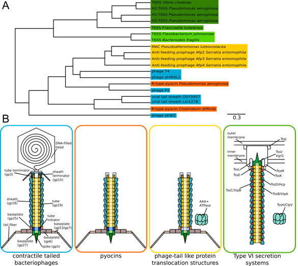
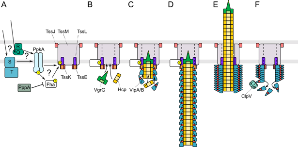
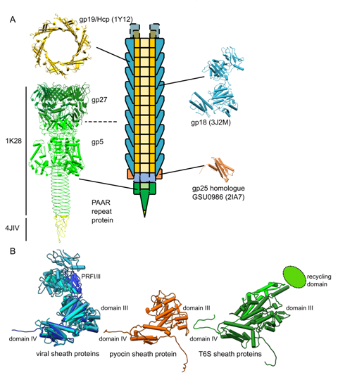
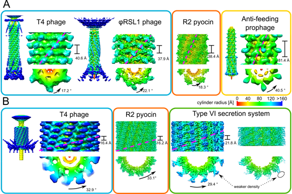
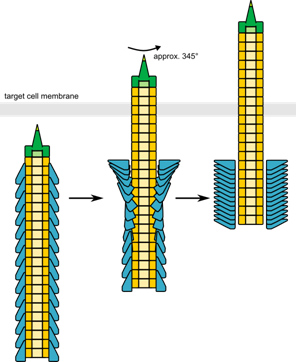

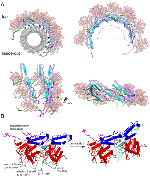
Figures(7) / Tables(2)

Sebastian Kube, Petra Wendler. Structural comparison of contractile nanomachines[J]. AIMS Biophysics, 2015, 2(2): 88-115. doi: 10.3934/biophy.2015.2.88

 DownLoad: