Quercus pyrenaica Willd thrives in the intermediate zone between the Mediterranean sclerophyllous and the temperate deciduous forest. In December 2022, the presence of the bacteria Xylella fastidiosa (Xf) was confirmed in samples collected from a Quercus pyrenaica located in Sabrosa, Vila Real, Portugal. Following Xf infection, the transport of water and nutrients is hindered due to the occlusion of xylem vessels. This loss of hydraulic conductivity may lead to vessel blockage and subsequent embolism formation. The objective of this study was to investigate the interaction between Xf and Quercus pyrenaica tissues, as well as the mechanism by which the bacteria can spread through the plant's xylem vessels, ultimately resulting in the formation of vascular plugs. At the time of the sample collection (10 months post-detection), symptoms of Bacterial Leaf Scorch (BLS) began to appear. Examination of xylem vessels using both light and scanning electron microscopy (SEM) revealed the presence of various types of occlusions, predominantly tyloses. Additionally, fibrillar networks, gums, starch grains, and crystals were observed. The stem vessels exhibited significantly more occlusions compared to the leaves. Furthermore, individual bacterial cells were observed to be attached to the vessel wall. This implies that occlusions were primarily induced by tyloses and gums as a defensive response to the invasion of vascular pathogens, in addition to the pathogen itself. This study highlights the presence of starch grains in stems, which may function as a refilling mechanism, thereby preventing the loss of hydraulic conductivity in plants and potentially acting as a means to entrap the bacteria. These mechanisms exemplify the constitutive defense systems of the plant against Xf. Understanding the interaction between Xylella fastidiosa and Quercus pyrenaica is crucial, given that the latter species occupies nearly 95% of the natural distribution area of Portugal.
Citation: Talita Loureiro, Berta Gonçalves, Luís Serra, Ângela Martins, Isabel Cortez, Patrícia Poeta. Histological analysis of Xylella fastidiosa infection in Quercus pyrenaica in Northern Portugal[J]. AIMS Agriculture and Food, 2024, 9(2): 607-627. doi: 10.3934/agrfood.2024033
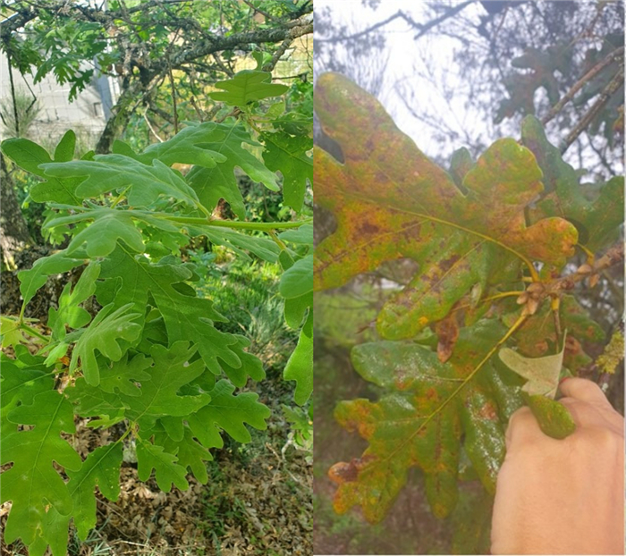
Quercus pyrenaica Willd thrives in the intermediate zone between the Mediterranean sclerophyllous and the temperate deciduous forest. In December 2022, the presence of the bacteria Xylella fastidiosa (Xf) was confirmed in samples collected from a Quercus pyrenaica located in Sabrosa, Vila Real, Portugal. Following Xf infection, the transport of water and nutrients is hindered due to the occlusion of xylem vessels. This loss of hydraulic conductivity may lead to vessel blockage and subsequent embolism formation. The objective of this study was to investigate the interaction between Xf and Quercus pyrenaica tissues, as well as the mechanism by which the bacteria can spread through the plant's xylem vessels, ultimately resulting in the formation of vascular plugs. At the time of the sample collection (10 months post-detection), symptoms of Bacterial Leaf Scorch (BLS) began to appear. Examination of xylem vessels using both light and scanning electron microscopy (SEM) revealed the presence of various types of occlusions, predominantly tyloses. Additionally, fibrillar networks, gums, starch grains, and crystals were observed. The stem vessels exhibited significantly more occlusions compared to the leaves. Furthermore, individual bacterial cells were observed to be attached to the vessel wall. This implies that occlusions were primarily induced by tyloses and gums as a defensive response to the invasion of vascular pathogens, in addition to the pathogen itself. This study highlights the presence of starch grains in stems, which may function as a refilling mechanism, thereby preventing the loss of hydraulic conductivity in plants and potentially acting as a means to entrap the bacteria. These mechanisms exemplify the constitutive defense systems of the plant against Xf. Understanding the interaction between Xylella fastidiosa and Quercus pyrenaica is crucial, given that the latter species occupies nearly 95% of the natural distribution area of Portugal.

| [1] |
Wells JM, Raju BC, Hung H-Y, et al. (1987) Xylella fastidiosa gen. nov., sp. nov: Gram-negative, xylem-limited, fastidious plant bacteria related to Xanthomonas spp. Int J Syst Evol Microbiol 37: 136–143. https://doi.org/10.1099/00207713-37-2-136 doi: 10.1099/00207713-37-2-136

|
| [2] | Pereira PS (2015) Xylella fastidiosa—A new menace for Portuguese agriculture and forestry. Revista de Ciências Agrárias (Portugal) 38: 149–154. |
| [3] |
Montilon V, De Stradis A, Saponari M, et al. (2023) Xylella fastidiosa subsp. pauca ST53 exploits pit membranes of susceptible olive cultivars to spread systemically in the xylem. Plant Pathol 72: 144–153. https://doi.org/10.1111/ppa.13646 doi: 10.1111/ppa.13646
|
| [4] | Petit G, Bleve G, Gallo A, et al. (2021) Susceptibility to Xylella fastidiosa and functional xylem anatomy in Olea europaea: Revisiting a tale of plant-pathogen interaction. AoB Plants 13: plab027. https://doi.org/10.1093/aobpla/plab027 |
| [5] |
Loureiro T, Mesquita MM, De Lurdes M, et al. (2023) Xylella fastidiosa: A glimpse of the Portuguese situation. Microbiol Res 14: 1568–1588. https://doi.org/10.3390/microbiolres14040108 doi: 10.3390/microbiolres14040108
|
| [6] | DGAV (2022) Plano de Contingência Xylella fastidiosa e seus vetores. |
| [7] |
Cavalieri V, Altamura G, Fumarola G, et al. (2019) Transmission of Xylella fastidiosa subspecies Pauca sequence type 53 by different insect species. Insects 10: 324. https://doi.org/10.3390/insects10100324 doi: 10.3390/insects10100324
|
| [8] |
Surano A, Abou Kubaa R, Nigro F, et al. (2022) Susceptible and resistant olive cultivars show differential physiological response to Xylella fastidiosa infections. Front Plant Sci 13: 968934. https://doi.org/10.3389/fpls.2022.968934 doi: 10.3389/fpls.2022.968934
|
| [9] |
Cornara D, Bosco D, Fereres A (2018) Philaenus spumarius: When an old acquaintance becomes a new threat to European agriculture. J Pest Sci 91: 957–972. https://doi.org/10.1007/s10340-018-0966-0 doi: 10.1007/s10340-018-0966-0
|
| [10] |
Calvo L, Santalla S, Marcos E, et al. (2003) Regeneration after wildfire in communities dominated by Pinus pinaster, an obligate seeder, and in others dominated by Quercus pyrenaica, a typical resprouter. For Ecol Manage 184: 209–223. https://doi.org/10.1016/S0378-1127(03)00207-X doi: 10.1016/S0378-1127(03)00207-X
|
| [11] | Castro M, Castro J, Gómez Sal A (2004) The role of black oak woodlands (Quercus pyrenaica Willd.) in small ruminant production in Northeast Portugal. Sustainability Agrosilvopastoral Systems, 221–229. |
| [12] | Chalmin A, Burgess P, Smith J, et al. (2014) EURAF EUROPEAN AGROFORESTRY FEDERATION: 2 nd European Agroforestry Conference—Integrating Science and Policy to Promote Agroforestry in Practice. Available from: https://www.repository.utl.pt/bitstream/10400.5/6764/1/REP-ⅡEURAF_Conference_Book_of_Abstracts.pdf |
| [13] | Carvalho A(2020) Plano de ação para erradicação de Xylella fastidiosa e controlo dos seus vetores—Zona demarcada. Plano de ação para controlo de Xylella fastidiosa. |
| [14] |
Scortichini M (2023) PM 7/24 (5) Xylella fastidiosa. EPPO Bulletin 53: 205–276. https://doi.org/10.1111/epp.12913 doi: 10.1111/epp.12913
|
| [15] | Kraus JE, Arduin M (1997) Manual básico de métodos em morfologia vegetal. |
| [16] | Conn HJ (1953) Biological stains: A handbook on the nature and uses of the dyes employed in the biological laboratory. https://doi.org/10.5962/bhl.title.5903 |
| [17] |
Inch S, Ploetz R, Held B, et al. (2012) Histological and anatomical responses in avocado, Persea americana, induced by the vascular wilt pathogen, Raffaelea lauricola. Botany 90: 627–635. https://doi.org/10.1139/b2012-015 doi: 10.1139/b2012-015
|
| [18] |
Sun Q, Rost TL, Matthews MA (2006) Pruning-induced tylose development in stems of current-year shoots of Vitis vinifera (Vitaceae). Am J Bot 93: 1567–1576. https://doi.org/10.3732/ajb.93.11.1567 doi: 10.3732/ajb.93.11.1567
|
| [19] | Lin H, Walker A (2004) Characterization and identification of Pierce's disease resistance mechanisms: Analysis of xylem anatomical structures and of natural products in xylem sap among Vitis. In: Pierce's Disease Research Symposium Proceedings, California Department of Food and Agriculture. San Diego, CA, USA, 22–24. |
| [20] |
Bouamama-Gzara B, Zemni H, Sleimi N, et al. (2022) Diversification of vascular occlusions and crystal deposits in the xylem sap flow of five Tunisian grapevines. Plants 11: 2177. https://doi.org/10.3390/plants11162177 doi: 10.3390/plants11162177
|
| [21] |
Fritschi FB, Lin H, Walker MA (2008) Scanning electron microscopy reveals different response pattern of four Vitis genotypes to Xylella fastidiosa infection. Plant Dis 92: 276–286. https://doi.org/10.1094/PDIS-92-2-0276 doi: 10.1094/PDIS-92-2-0276
|
| [22] | Cardinale M, Luvisi A, Meyer JB, et al. (2018) Specific fluorescence in situ hybridization (Fish) test to highlight colonization of xylem vessels by Xylella fastidiosa in naturally infected olive trees (Olea europaea L.). Front Plant Sci 9: 431. https://doi.org/10.3389/fpls.2018.00431 |
| [23] |
De Benedictis M, De Caroli M, Baccelli I, et al. (2017) Vessel occlusion in three cultivars of Olea europaea naturally exposed to Xylella fastidiosa in open field. J Phytopathol 165: 589–594. https://doi.org/10.1111/jph.12596 doi: 10.1111/jph.12596
|
| [24] |
Sun Q, Sun Y, Andrew Walker M, et al. (2013) Vascular occlusions in grapevines with Pierce's disease make disease symptom development worse. Plant Physiol 161: 1529–1541. https://doi.org/10.1104/pp.112.208157 doi: 10.1104/pp.112.208157
|
| [25] |
De Micco V, Balzano A, Wheeler EA, et al. (2016) Tyloses and gums: A review of structure, function and occurrence of vessel occlusions. IAWA J 37: 186–205. https://doi.org/10.1163/22941932-20160130 doi: 10.1163/22941932-20160130
|
| [26] |
Mcelrone AJ, Jackson S, Habdas P (2008) Hydraulic disruption and passive migration by a bacterial pathogen in oak tree xylem. J Exp Bot 59: 2649–2657. https://doi.org/10.1093/jxb/ern124 doi: 10.1093/jxb/ern124
|
| [27] | Tyree MT, Zimmermann MH (2002) Xylem Structure and the Ascent of Sap. 283. https://doi.org/10.1007/978-3-662-04931-0 |
| [28] |
Cochard H, Tyree MT (1990) Xylem dysfunction in Quercus: Vessel sizes, tyloses, cavitation and seasonal changes in embolism. Tree Physiol 6: 393–407. https://doi.org/10.1093/treephys/6.4.393 doi: 10.1093/treephys/6.4.393
|
| [29] |
Queiroz-Voltan RB, Perosin Cabral L, Paradela Filho O (2004) Severidade do sintoma da bactéria Xylella fastidiosa em cultivares de cafeeiro. Bragantia 63: 395–404. https://doi.org/10.1590/S0006-87052004000300009 doi: 10.1590/S0006-87052004000300009
|
| [30] |
Stevenson JF, Matthews MA, Greve LC, et al. (2004) Grapevine susceptibility to Pierce's disease Ⅱ: Progression of anatomical symptoms. Am J Enol Vitic 55: 238–245. https://doi.org/10.5344/ajev.2004.55.3.238 doi: 10.5344/ajev.2004.55.3.238
|
| [31] |
Baccari C, Lindow SE (2010) Assessment of the process of movement of Xylella fastidiosa within susceptible and resistant grape cultivars. Phytopathology 101: 77–84. https://doi.org/10.1094/PHYTO-04-10-0104 doi: 10.1094/PHYTO-04-10-0104
|
| [32] |
Roper MC, Greve LC, Warren JG, et al. (2007) Xylella fastidiosa requires polygalacturonase for colonization and pathogenicity in Vitis vinifera grapevines. Mol Plant Microbe Interact 20: 411–419. https://doi.org/10.1094/MPMI-20-4-0411 doi: 10.1094/MPMI-20-4-0411
|
| [33] |
Giovannoni M, Gramegna G, Benedetti M, et al. (2020) Industrial use of cell wall degrading enzymes: The fine line between production strategy and economic feasibility. Front Bioeng Biotechnol 8: 529626. https://doi.org/10.3389/fbioe.2020.00356 doi: 10.3389/fbioe.2020.00356
|
| [34] |
Newman KL, Almeida RPP, Purcell AH, et al. (2004) Cell-cell signaling controls Xylella fastidiosa interactions with both insects and plants. Proc Natl Acad Sci USA 101: 1737–1742. https://doi.org/10.1073/pnas.0308399100 doi: 10.1073/pnas.0308399100
|
| [35] |
Clara Fanton A, Brodersen C (2021) Hydraulic consequences of enzymatic breakdown of grapevine pit membranes. Plant Physiol 186: 1919. https://doi.org/10.1093/plphys/kiab191 doi: 10.1093/plphys/kiab191
|
| [36] |
Pérez-Donoso AG, Lenhof JJ, Pinney K, et al. (2016) Vessel embolism and tyloses in early stages of Pierce's disease. Aust J Grape Wine Res 22: 81–86. https://doi.org/10.1111/ajgw.12178 doi: 10.1111/ajgw.12178
|
| [37] |
Ingel B, Reyes C, Massonnet M, et al. (2021) Xylella fastidiosa causes transcriptional shifts that precede tylose formation and starch depletion in xylem. Mol Plant Pathol 22: 175–188. https://doi.org/10.1111/mpp.13016 doi: 10.1111/mpp.13016
|
| [38] |
Pérez-Donoso AG, Sun Q, Caroline Roper M, et al. (2010) Cell wall-degrading enzymes enlarge the pore size of intervessel pit membranes in healthy and Xylella fastidiosa-infected grapevines. Plant Physiol 152: 1748–1759. https://doi.org/10.1104/pp.109.148791 doi: 10.1104/pp.109.148791
|
| [39] |
Brodersen CR, McElrone AJ (2013) Maintenance of xylem network transport capacity: A review of embolism repair in vascular plants. Front Plant Sci 4: 47335. https://doi.org/10.3389/fpls.2013.00108 doi: 10.3389/fpls.2013.00108
|
| [40] |
Roper MC, Greve LC, Labavitch JM, et al. (2007) Detection and visualization of an exopolysaccharide produced by Xylella fastidiosa in vitro and in planta. Appl Environ Microbiol 73: 7252–7258. https://doi.org/10.1128/AEM.00895-07 doi: 10.1128/AEM.00895-07
|
| [41] |
Newman KL, Almeida RPP, Purcell AH, et al. (2003) Use of a green fluorescent strain for analysis of Xylella fastidiosa colonization of Vitis vinifera. Appl Environ Microbiol 69: 7319–7327. https://doi.org/10.1128/AEM.69.12.7319-7327.2003 doi: 10.1128/AEM.69.12.7319-7327.2003
|
| [42] |
Falsini S, Tani C, Sambuco G, et al. (2022) Anatomical and biochemical studies of Spartium junceum infected by Xylella fastidiosa subsp. multiplex ST 87. Protoplasma 259: 103–115. https://doi.org/10.1007/s00709-021-01640-2 doi: 10.1007/s00709-021-01640-2
|
| [43] |
Sabella E, Aprile A, Genga A, et al. (2019) Xylem cavitation susceptibility and refilling mechanisms in olive trees infected by Xylella fastidiosa. Sci Rep 9: 9602. https://doi.org/10.1038/s41598-019-46092-0 doi: 10.1038/s41598-019-46092-0
|
| [44] |
Van Ieperen W, Van Meeteren U, Van Gelder H (2000) Fluid ionic composition influences hydraulic conductance of xylem conduits. J Exp Bot 51: 769–776. https://doi.org/10.1093/jexbot/51.345.769 doi: 10.1093/jexbot/51.345.769
|
| [45] |
Chatelet DS, Wistrom CM, Purcell AH, et al. (2011) Xylem structure of four grape varieties and 12 alternative hosts to the xylem-limited bacterium Xylella fastidious. Ann Bot 108: 73–85. https://doi.org/10.1093/aob/mcr106 doi: 10.1093/aob/mcr106
|
| [46] |
Pouzoulet J, Scudiero E, Schiavon M, et al. (2017) Xylem vessel diameter affects the compartmentalization of the vascular pathogen phaeomoniella chlamydospora in grapevine. Front Plant Sci 8: 281014. https://doi.org/10.3389/fpls.2017.01442 doi: 10.3389/fpls.2017.01442
|
| [47] | De Souza AA, Takita MA, Amaral A, et al. (2009) Citrus responses to Xylella fastidiosa infection, the causal agent of citrus variegated chlorosis. Tree For Sci Biotechnol 3: 73–80. |
| [48] |
Leite B, Ishida ML, Alves E, et al. (2002) Genomics and X-ray microanalysis indicate that Ca2+ and thiols mediate the aggregation and adhesion of Xylella fastidiosa. Braz J Med Biol Res 35: 645–650. https://doi.org/10.1590/S0100-879X2002000600003 doi: 10.1590/S0100-879X2002000600003
|
| [49] |
Pinheiro C, Chaves MM (2011) Photosynthesis and drought: can we make metabolic connections from available data? J Exp Bot 62: 869–882. https://doi.org/10.1093/jxb/erq340 doi: 10.1093/jxb/erq340
|
| [50] |
McDowell NG (2011) Mechanisms linking drought, hydraulics, carbon metabolism, and vegetation mortality. Plant Physiol 155: 1051–1059. https://doi.org/10.1104/pp.110.170704 doi: 10.1104/pp.110.170704
|
| [51] |
Valtaud C, Foyer CH, Fleurat-Lessard P, et al. (2009) Systemic effects on leaf glutathione metabolism and defence protein expression caused by esca infection in grapevines. Funct Plant Biol 36: 260–279. https://doi.org/10.1071/FP08293 doi: 10.1071/FP08293
|
| [52] |
A, Lo Gullo MA, Salleo S (2011) Refilling embolized xylem conduits: Is it a matter of phloem unloading? Plant Sci 180: 604–611. https://doi.org/10.1016/j.plantsci.2010.12.011 doi: 10.1016/j.plantsci.2010.12.011
|
| [53] |
Masrahi YS (2014) Ecological significance of wood anatomy in two lianas from arid southwestern Saudi Arabia. Saudi J Biol Sci 21: 334–341. https://doi.org/10.1016/j.sjbs.2013.11.005 doi: 10.1016/j.sjbs.2013.11.005
|
| [54] |
Bucci SJ, Scholz FG, Goldstein G, et al. (2003) Dynamic changes in hydraulic conductivity in petioles of two savanna tree species: factors and mechanisms contributing to the refilling of embolized vessels. Plant Cell Environ 26: 1633–1645. https://doi.org/10.1046/j.0140-7791.2003.01082.x doi: 10.1046/j.0140-7791.2003.01082.x
|
| [55] | European Food Safety Authority (EFSA), Gibin D, Pasinato L, et al. (2023) Update of the Xylella spp. host plant database—Systematic literature search up to 31 December 2022. EFSA J 21: e08061. https://doi.org/10.2903/j.efsa.2023.8061 |


Figures(7)

Talita Loureiro, Berta Gonçalves, Luís Serra, Ângela Martins, Isabel Cortez, Patrícia Poeta. Histological analysis of Xylella fastidiosa infection in Quercus pyrenaica in Northern Portugal[J]. AIMS Agriculture and Food, 2024, 9(2): 607-627. doi: 10.3934/agrfood.2024033


 DownLoad: