Comparison of eleven measures for estimating difficulty of open-loop TSP instances

Lahari Sengupta; Pasi Fränti; Lahari Sengupta; Pasi Fränti

doi:10.3934/aci.2021001

Applied Computing and Intelligence

2021, Volume 1, Issue 1: 1-30. doi: 10.3934/aci.2021001

Previous Article Next Article

Review

Comparison of eleven measures for estimating difficulty of open-loop TSP instances

Lahari Sengupta ,
Pasi Fränti ^,

Machine Learning, School of Computing, University of Eastern Finland, Finland

Academic Editor: Chih-Cheng Hung

Received: 11 August 2021 Accepted: 13 September 2021 Published: 23 September 2021

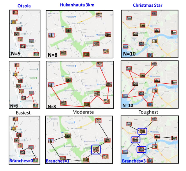
From the theory of algorithms, we know that the time complexity of finding the optimal solution for a traveling salesman problem (TSP) grows exponentially with the number of targets. However, the size of the problem instance is not the only factor that affects its difficulty. In this paper, we review existing measures to estimate the difficulty of a problem instance. We also introduce MST branches and two other measures called greedy path and greedy gap. The idea of MST branches is to generate minimum spanning tree (MST) and then calculate the number of branches in the tree. A branch is a target, which is connected to at least two other targets. We perform an extensive comparison of 11 measures to see how well they correlate to human and computer performance. We evaluate the measures based on time complexity, prediction capability, suitability, and practicality. The results show that while the MST branches measure is simple, fast to compute, and does not need to have the optimal solution as a reference unlike many other measures. It correlates equally good or even better than the best of the previous measures ‑ the number of targets, and the number of targets on the convex hull.
- TSP,
- open-loop TSP,
- difficulty of instances,
- MST,
- human TSP solving
Citation: Lahari Sengupta, Pasi Fränti. Comparison of eleven measures for estimating difficulty of open-loop TSP instances[J]. Applied Computing and Intelligence, 2021, 1(1): 1-30. doi: 10.3934/aci.2021001

Related Papers:

Abstract

From the theory of algorithms, we know that the time complexity of finding the optimal solution for a traveling salesman problem (TSP) grows exponentially with the number of targets. However, the size of the problem instance is not the only factor that affects its difficulty. In this paper, we review existing measures to estimate the difficulty of a problem instance. We also introduce MST branches and two other measures called greedy path and greedy gap. The idea of MST branches is to generate minimum spanning tree (MST) and then calculate the number of branches in the tree. A branch is a target, which is connected to at least two other targets. We perform an extensive comparison of 11 measures to see how well they correlate to human and computer performance. We evaluate the measures based on time complexity, prediction capability, suitability, and practicality. The results show that while the MST branches measure is simple, fast to compute, and does not need to have the optimal solution as a reference unlike many other measures. It correlates equally good or even better than the best of the previous measures ‑ the number of targets, and the number of targets on the convex hull.

References

[1]	Papadimitriou CH, The Euclidean travelling salesman problem is NP-complete. Theoretical Computer Science, 4(3), 237-244, 1977. doi: 10.1016/0304-3975(77)90012-3 doi: 10.1016/0304-3975(77)90012-3
[2]	Phillips N and Phillips R, Rogaining: Cross-Country Navigation. Outdoor Recreation in Australia. ISBN 0-9593329-2-8.
[3]	Fränti P, Mariescu-Istodor R, and Sengupta L, O-Mopsi: Mobile Orienteering Game for Sightseeing, Exercising, and Education. ACM Transactions on Multimedia Computing, Communications, and Applications, 13(4), 56, 1-12, 2017. doi: 10.1145/3115935
[4]	Sengupta L and Fränti P, Predicting the difficulty of TSP instances using MST. IEEE Int. Conf. on Industrial Informatics (INDIN), pp. 847-852, Helsinki 2019.
[5]	Vickers D, Mayo T, Heitmann M, Lee MD, and Hughes P, Intelligence and individual differences on three types of visually presented optimisation problems. Personality and Individual Differences, 36, 1059-1071, 2004. doi:10.1016/S0191-8869(03)00200-9 doi: 10.1016/S0191-8869(03)00200-9
[6]	Dry MJ, Preiss K, and Wagemans J, Clustering, Randomness, and Regularity: Spatial Distributions and Human Performance on the Traveling Salesperson Problem and Minimum Spanning Tree Problem. The Journal of Problem Solving, 4(1), 2, 2012. doi: 10.7771/1932-6246.1117 doi: 10.7771/1932-6246.1117
[7]	Graham SM, Joshi A, and Pizlo Z, The traveling salesman problem: A hierarchical model. Memory and Cognition, 28(7), 1191-1204, 2000. doi: 10.3758/BF03211820 doi: 10.3758/BF03211820
[8]	Dry MJ, Lee MD, Vickers D, and Hughes P, Human performance on visually presented traveling salesperson problems with varying numbers of nodes. Journal of Problem Solving, 1(1), 4, 2006. doi: 10.7771/1932-6246.1004
[9]	Macgregor JN and Ormerod T, Human performance on the traveling salesman problem. Perception and Psychophysics 58: 527-539, 1996. doi: 10.3758/BF03213088
[10]	Chronicle EP, MacGregor JN, Ormerod TC, and Burr A, It looks easy! Heuristics for combinatorial optimisation problems. Quarterly Journal of Experimental Psychology, 59,783–800, 2006. doi: 10.1080/02724980543000033 doi: 10.1080/02724980543000033
[11]	Fischer T, Stützle T, Hoos H, and Merz P, An analysis of the hardness of TSP instances for two high performance algorithms. Metaheuristics International Conference, pp. 361-367, 2005.
[12]	Applegate D, Bixby R, Chvátal V, and Cook W, Implementing the Dantzig-Fulkerson-Johnson algorithm for large traveling salesman problems. Mathematical Programming, 97, 91-153, 2003. doi: 10.1007/s10107-003-0440-4 doi: 10.1007/s10107-003-0440-4
[13]	Helsgaun K, An effective implementation of the Lin–Kernighan traveling salesman heuristic. European Journal of Operational Research, 126(1), 106-130, 2000. doi 10.1016/S0377-2217(99)00284-2 doi: 10.1016/S0377-2217(99)00284-2
[14]	Leyton-Brown K, Hoos HH, Hutter F, and Xu L, Understanding the empirical hardness of NP-complete problems. Communications of the ACM, 57(5), 98-107, 2014. doi: 10.1145/2594413.2594424 doi: 10.1145/2594413.2594424
[15]	Kromer P, Platos J, and Kudelka M, Network measures and evaluation of traveling salesman instance hardness. IEEE Symposium Series on Computational Intelligence (SSCI), pp. 1-7, Honululu, 2017.
[16]	Ochodkova E, Zehnalova S, and Kudelka M, Graph construction based on local representativeness. International Computing and Combinatorics Conference, pp 654-665. Springer, Cham, 2017.
[17]	Vickers D, Lee MD, Dry M, Hughes P, and McMahon JA, The aesthetic appeal of minimal structures: Judging the attractiveness of solutions to traveling salesperson problems. Perception and Psychophysics, 68 (1), 32-42, 2006. doi: 10.3758/BF03193653 doi: 10.3758/BF03193653
[18]	MacGregor JN, Indentations and starting points in traveling sales tour problems: Implications for theory. Journal of Problem Solving, 5(1), 2–17, 2012. doi: 10.7771/1932-6246.1140 doi: 10.7771/1932-6246.1140
[19]	Vickers D, Lee MD, Dry M, and Hughes P, The roles of the convex hull and the number of potential intersections in performance on visually presented traveling salesperson problems. Memory and Cognition, 31(7), 1094-1104, 2003. doi: 10.3758/bf03196130 doi: 10.3758/bf03196130
[20]	Kruskal JB, On the shortest spanning subtree of a graph and the traveling salesman problem. Proceedings of the American Mathematical society, 7(1), 48-50, 1956. doi: 10.1090/S0002-9939-1956-0078686-7 doi: 10.1090/S0002-9939-1956-0078686-7
[21]	Prim RC, Shortest connection networks and some generalizations. The Bell System Technical Journal, 36(6), 1389-1401, 1957. doi: 10.1002/j.1538-7305.1957.tb01515.x doi: 10.1002/j.1538-7305.1957.tb01515.x
[22]	Christofides N, Worst-case analysis of a new heuristic for the travelling salesman problem, Report 388, Graduate School of Industrial Administration, CMU, 1976.
[23]	Rosenkrantz J, Stearns RE, Lewis II PM, An analysis of several heuristics for the travelling salesman problem, SIAM journal on Computing, 6,563-581, 1977. doi: 10.1137/0206041 doi: 10.1137/0206041
[24]	Fränti P and Nenonen H, Modifying Kruskal algorithm to solve open loop TSP. Multidisciplinary International Scheduling Conference (MISTA), pp. 584-590, Ningbo, China, 2019.
[25]	Fränti P, Nenonen T, and Yuan M, Converting MST to TSP path by branch elimination, Applied Sciences, 11(177), 1-17, 2021. doi: 10.3390/app11010177 doi: 10.3390/app11010177
[26]	Laporte G, The traveling salesman problem: An overview of exact and approximate algorithms. European Journal of Operational Research, 59(2), 231-247, 1992. doi: 10.1016/0377-2217(92)90138-Y
[27]	Sengupta L, Mariescu-Istodor R, and Fränti P, Planning your route: Where to start?. Computational Brain and Behavior, 1(3), 252-265, 2018. doi: 10.1007/s42113-018-0018-0 doi: 10.1007/s42113-018-0018-0
[28]	MacGregor JN, Chronicle EP, and Ormerod TC, Convex hull or crossing avoidance? Solution heuristics in the traveling salesperson problem. Memory and Cognition, 32(2), 260-270, 2004. doi: 10.3758/bf03196857 doi: 10.3758/bf03196857
[29]	Mariescu-Istodor R and Fränti P, Solving large-scale TSP problem in 1 hour: Santa Claus Challenge 2020. Frontiers in Robotics and AI (submitted), 2021.
[30]	Andrew AM, Another efficient algorithm for convex hulls in two dimensions. Information Processing Letters, 9(5), 216-219, 1979. doi: 10.1016/0020-0190(79)90072-3 doi: 10.1016/0020-0190(79)90072-3
[31]	Ormerod TC, Chronicle EP, Global perceptual processing in problem solving: The case of the traveling salesperson. Perception and Psychophysics 61, 1227–1238, 1999. doi: 10.3758/bf03207625
[32]	Dry MJ and Fontaine EL, Fast and efficient discrimination of traveling salesperson problem stimulus difficulty. The Journal of Problem Solving, 7(1), 9, 2014. doi: 10.7771/1932-6246.1160 doi: 10.7771/1932-6246.1160
[33]	Braden B, The surveyor's area formula. The College Mathematics Journal, 17(4), 326-337, 1986. doi: 10.1080/07468342.1986.11972974 doi: 10.1080/07468342.1986.11972974
[34]	Applegate DL, Bixby RE, Chvatal V, and Cook WJ, The traveling salesman problem: a computational study. Princeton University Press, 2011
[35]	Quintas LV, Supnick F, Extreme Hamiltonian circuits. Resolution of the convex-even case. Proceedings of the American Mathematical Society, 16(5), 1058-1061, 1965. doi: 10.2307/2035616
[36]	Van Rooij I, Stege U, and Schactman A, Convex hull and tour crossings in the Euclidean traveling salesperson problem: Implications for human performance studies. Memory and Cognition, 31(2), 215-220, 2003. doi: 10.3758/BF03194380 doi: 10.3758/BF03194380
[37]	Yang JQ, Yang JG, and Chen GL, Solving large-scale TSP using adaptive clustering method. IEEE International Symposium on Computational Intelligence and Design, 1, 49-51, 2009. doi: 10.1109/ISCID.2009.19 doi: 10.1109/ISCID.2009.19
[38]	MacGregor JN, Effects of cluster location on human performance on the Traveling Salesperson Problem. The Journal of Problem Solving, 5(2), 3, 2013. doi: 10.7771/1932-6246.1151 doi: 10.7771/1932-6246.1151
[39]	Žunić J and Hirota K, Measuring shape circularity. Iberoamerican Congress on Pattern Recognition (pp. 94-101). Springer, Berlin, Heidelberg, 2008.
[40]	Schick A, Fischer M, and Stiefelhagen R, Measuring and evaluating the compactness of superpixels. International Conference on Pattern Recognition (ICPR), pp. 930-934, IEEE, 2012.
[41]	Sengupta L, Mariescu-Istodor R, and Fränti P, Which local search operator works best for the open-loop TSP? Applied Sciences, 9(19), 3985, 2019. doi: 10.3390/app9193985
[42]	Jormanainen I and Korhonen P, Science festivals on computer science recruitment. Koli Calling International Conference on Computing Education Research (Koli Calling'10). ACM, New York, 72–73, 2010.
[43]	MacGregor JN, Ormerod TC, and Chronicle EP, Spatial and contextual factors in human performance on the travelling salesperson problem. Perception. 28(11): 1417-1427, 1999. doi: 10.1068/p2863
[44]	MacGregor JN, Ormerod TC, and Chronicle EP, A model of human performance on the traveling salesperson problem. Memory and Cognition. 28: 1183-1190, 2000. doi: 10.3758/BF03211819
[45]	Zhao Q and Fränti P, WB-index: A sum-of-squares based index for cluster validity. Data & Knowledge Engineering, 92, 77-89, 2014. doi: 10.1016/j.datak.2014.07.008 doi: 10.1016/j.datak.2014.07.008

Reader Comments

Your name:*

Email:*
© 2021 the Author(s), licensee AIMS Press. This is an open access article distributed under the terms of the Creative Commons Attribution License (http://creativecommons.org/licenses/by/4.0)