A naive justification of hyperbolic discounting from mental algebraic operations and functional analysis

Salvador Cruz Rambaud; Jorge Hernandez-Perez; Salvador Cruz Rambaud; Jorge Hernandez-Perez

doi:10.3934/QFE.2023023

Quantitative Finance and Economics

2023, Volume 7, Issue 3: 463-474. doi: 10.3934/QFE.2023023

Previous Article Next Article

Research article

A naive justification of hyperbolic discounting from mental algebraic operations and functional analysis

Departamento de Economía y Empresa, University of Almería, La Cañada de San Urbano, s/n, 04120, Almería, Spain

Received: 09 July 2023 Revised: 27 August 2023 Accepted: 08 September 2023 Published: 14 September 2023
JEL Codes: C02, D91, G40

Background

Intertemporal decision-making, which involves making choices between outcomes at different time points, is a fundamental aspect of human behavior. Understanding the underlying mental processes is vital for comprehending the complexities of human decision-making and choice behavior.

Objective

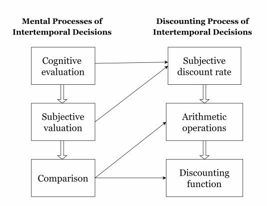
The main objective of this study is to investigate the interplay of mental processes, specifically cognitive evaluation, subjective valuation, and comparison, in the context of intertemporal decision-making, with a specific focus on understanding the discounting process.

Methodology

Development of a mathematical representation of the discounting process that incorporates the mental processes associated with intertemporal decision-making.

Result

Our findings indicate that hyperbolic discounting aligns well with the cognitive processes underlying intertemporal decision-making. Subsequent research will employ qualitative questionnaires to establish the discount function relevant to specific groups, thereby enhancing our comprehension of the discounting process within intertemporal decision-making.

Keywords:

Citation: Salvador Cruz Rambaud, Jorge Hernandez-Perez. A naive justification of hyperbolic discounting from mental algebraic operations and functional analysis[J]. Quantitative Finance and Economics, 2023, 7(3): 463-474. doi: 10.3934/QFE.2023023

Related Papers:

[1]	Lorenza D'Elia . $\Gamma$ -convergence of quadratic functionals with non uniformly elliptic conductivity matrices. Networks and Heterogeneous Media, 2022, 17(1): 15-45. doi: 10.3934/nhm.2021022
[2]	Andrea Braides, Valeria Chiadò Piat . Non convex homogenization problems for singular structures. Networks and Heterogeneous Media, 2008, 3(3): 489-508. doi: 10.3934/nhm.2008.3.489
[3]	Patrick Henning . Convergence of MsFEM approximations for elliptic, non-periodic homogenization problems. Networks and Heterogeneous Media, 2012, 7(3): 503-524. doi: 10.3934/nhm.2012.7.503
[4]	Leonid Berlyand, Volodymyr Rybalko . Homogenized description of multiple Ginzburg-Landau vortices pinned by small holes. Networks and Heterogeneous Media, 2013, 8(1): 115-130. doi: 10.3934/nhm.2013.8.115
[5]	Manuel Friedrich, Bernd Schmidt . On a discrete-to-continuum convergence result for a two dimensional brittle material in the small displacement regime. Networks and Heterogeneous Media, 2015, 10(2): 321-342. doi: 10.3934/nhm.2015.10.321
[6]	Fabio Camilli, Claudio Marchi . On the convergence rate in multiscale homogenization of fully nonlinear elliptic problems. Networks and Heterogeneous Media, 2011, 6(1): 61-75. doi: 10.3934/nhm.2011.6.61
[7]	Brahim Amaziane, Leonid Pankratov, Andrey Piatnitski . Homogenization of variational functionals with nonstandard growth in perforated domains. Networks and Heterogeneous Media, 2010, 5(2): 189-215. doi: 10.3934/nhm.2010.5.189
[8]	Antonio DeSimone, Martin Kružík . Domain patterns and hysteresis in phase-transforming solids: Analysis and numerical simulations of a sharp interface dissipative model via phase-field approximation. Networks and Heterogeneous Media, 2013, 8(2): 481-499. doi: 10.3934/nhm.2013.8.481
[9]	Liselott Flodén, Jens Persson . Homogenization of nonlinear dissipative hyperbolic problems exhibiting arbitrarily many spatial and temporal scales. Networks and Heterogeneous Media, 2016, 11(4): 627-653. doi: 10.3934/nhm.2016012
[10]	Peter Bella, Arianna Giunti . Green's function for elliptic systems: Moment bounds. Networks and Heterogeneous Media, 2018, 13(1): 155-176. doi: 10.3934/nhm.2018007

Abstract

Background

Objective

Methodology

Development of a mathematical representation of the discounting process that incorporates the mental processes associated with intertemporal decision-making.

Result

1. Introduction

Natural hazards such as landslides and subsidence have been recognized as important impediments to developing nations' sustainable development ^[1,2,3,4]. For example, on December 20, 2015, in Guangming, Shenzhen, China, a catastrophic landfill slope landslide claimed the lives of 69 individuals ^[5]. Natural hazard risk assessment and management will have short-term benefits in terms of severity reduction and long-term benefits in terms of achieving sustainable development goals ^[1].

Slope stability evaluation is essential for analyzing and mitigating natural hazards in mountainous environments. Many attempts have been made to evaluate slope stability ^[6,7,8]. Owing to the inherent complexity and uncertainty, assessing slope stability for circular mode failure, a common problem, remains a challenge for practitioners and researchers ^[9]. Several methods for evaluating slope stability have been presented, with the limit equilibrium approach and numerical simulation method being the two most commonly used ^[10]. Limited equilibrium methods, such as the simplified Bishop, Spencer and Morgenstern-Price methods, are frequently implemented in practice. In general, soil material properties (unit weight, cohesion and friction angle) and the pore pressure ratio are required for limited equilibrium methods ^[11,12]. Numerical methods (e.g., finite element methods) have been extensively used to analyze slope stability. However, the major drawback is that their input parameters need to be back analyzed using in-situ measurements, which is not available in many cases ^[13]. Both methods have pros and cons. Finding the critical slip surface using the limit equilibrium method is difficult due to the large number of potential slip surfaces ^[14]. The numerical simulation method's accuracy is greatly influenced by the choice of constitutive models, mechanical parameters and boundary conditions, and it is frequently necessary to have a great deal of engineering expertise and to conduct on-site back analysis in order to make a reasonable choice and obtain reasonable results ^[15,16]. Consequently, predicting slope stability still presents considerable challenges.

In recent years, machine learning (ML) models have gained attention for solving very complex, nonlinear and multivariable geotechnical problems ^[17,18,19]. Assessments of slope stability circular failure using methods based on soft computing are summarized in Table 1. Despite their reliable and precise outputs, however, most algorithms are not readily applicable in practice owing to their complicated training and modeling procedures and "black box" aspects, i.e., these models do not demonstrate a transparent and understandable relationship between inputs and output. Quinlan ^[20] developed the model tree algorithm to get over these limitations. It integrates principles from decision trees and linear regression. In addition to the widespread application of soft computing techniques, several studies have only been conducted on a limited amount of data, which might restrict the classifier's ability to generalize. In the current study, an updated database of 627 cases comprising unit weight, cohesion, internal friction angle, slope angle and height, pore pressure ratio and stability status of circular mode failure has been compiled. To predict slope stability, a new logistic model tree (LMT) model is developed. This algorithm is an intelligent choice for classification and decision-making since it can solve the classification problem by combining a tree model and a logistic regression (LR) technique. Adding LR to the leaves of the tree allows for a probabilistic interpretation of the model's output, making it easier to explain, as they represent a series of if-then-else rules. The LMT has been employed in predicting pillar stability in geotechnical engineering ^[21], but it has not yet been used to predict slope stability.

Table 1. A summary of the ML-based circular mode failure assessment of slope stability.

Dataset (Stable/Failed)	Input parameters	Data Preprocessing	ML techniques	Reference
422 (226/196)	γ, c, ϕ, β, H, r_u	Data normalization	MDMSE	Zhang et al. ^[22]
444 (224/220)	γ, c, ϕ, β, H, r_u	Data normalization	AdaBoost, GBM Bagging, XRT, RF, HGB Voting Stacked	Lin et al. ^[23]
19 (13/6)	γ, c, ϕ, β, H, r_u	Data normalization	K-means cluster	Haghshenas et al. ^[24]
153 (83/70)	γ, c, ϕ, β, H, r_u	Data normalization and outlier removing	KNN, SVM, SGD, GP, QDA, GNB, DT, ANN, Bagging ensemble, Heterogeneous ensemble	Pham et al. ^[25]
257 (123/134)	γ, c, ϕ, β, H, r_u	–	XGB, RF, LR, SVM, BC, LDA, KNN, DT, MLP, GNB, XRT, Stacked ensemble	Kardani et al. ^[26]
87 (42/45)	γ, c, ϕ, β, H, r_u	–	J48	Amirkiyaei and Ghasemi ^[27]
221 (115/106)	γ, c, ϕ, β, H, r_u	Data normalization	ANN, SVM, RF, GBM	Zhou et al. ^[28]
148 (78/70)	γ, c, ϕ, β, H, r_u	Data normalization	LR, DT, RF, GBM, SVM, BP	Qi and Tang ^[29]
168 (84/84)	γ, c, ϕ, β, H, r_u	Data normalization	GP, QDA, SVM, ADB-DT, ANN, KNN Classifier ensemble	Qi and Tang ^[15]
107 (48/59)	γ, c, ϕ, β, H, r_u	–	RF, SVM, Bayes, GSA	Lin et al. ^[30]
82 (49/33)	γ, c, ϕ, β, H, r_u	–	NB	Feng et al. ^[31]
168 (84/84)	γ, c, ϕ, β, H, r_u	Data normalization	RBF, LSSVM, ELM	Hoang and Bui ^[32]
168 (84/84)	γ, c, ϕ, β, H, r_u	Data normalization	LSSVM	Hoang and Pham ^[33]
46 (17/29)	γ, c, ϕ, β, H, r_u	Data normalization	SVM	Xue et al. ^[34]
32 (14/18)	γ, c, ϕ, β, H, r_u	–	ANN	Lu and Rosenbaum ^[35]
82 (38/44)	γ, c, ϕ, β, H, r_u	–	BP	Feng ^[36]
Note: MDMSE-margin distance minimization selective ensemble, AdaBoost-adaptive boosting, GBM-gradient boosting machine, XRT-extremely randomized tree, RF-random forest, HGB-hist gradient boosting classifier, KNN-k-nearest neighbors, SVM-support vector machine, SGD-stochastic gradient descent, GP-Gaussian process, QDA-quadratic discriminant analysis, GNB-Gaussian naive Bayes, DT-decision tree, ANN-artificial neural network, XGB-extreme gradient boosting, BC-bagging classifier, LDA-linear discriminant analysis, MLP-multilayer perceptron, BP-back-propagation, QDA-quadratic discriminant analysis, ADB-DT-adaptive boosted decision tree, GSA-gravitational search algorithm, NB-naive Bayes, RBF-radial basis function, LSSVM-least squares support vector machine, ELM-extreme learning machine, γ-unit weight, c-cohesion, ϕ-angle of internal friction, β-slope angle, H-slope height, r_u-pore pressure ratio.

| Show Table

DownLoad: CSV

2. Materials and methods

2.1. LMT

LR is a straightforward method with features such as stability, low variance and time-efficient training ^[37], but its prediction outputs are frequently biased. Decision trees are another ML technique for searching a less confined space of candidate models and obtaining nonlinear patterns from a database; they have low bias but high variance and instability, making them susceptible to overfitting. Landwehr et al. ^[38] presented the LMT methodology as a result. It is based on Quinlan's model tree approach ^[20] for dealing with regression problems by combining linear regression with decision tree models, and it is extended to classification problems. This section provides a basic introduction to LMT, whereas the seminal work by Landwehr et al. ^[38] provides a more complete description.

2.2. Tree structure

A LR tree with LR functions built at the leaves constitutes an LMT. It has a set of leaves or terminal nodes T and an inner or non-terminal node set N. Each leaf t of the LMT model has correlated LR functions instead of classification labels or linear regression functions. The output vector is Y, and the input vector X is (X₁, X₂), for instance. S represents the complete instance space, which can be further partitioned into numerous subspaces S_t. Figure 1 displays a simple input space that has been partitioned into seven subspaces.

Figure 1. The input space is separated into seven subspaces (solid circles and square points represent different classes within the same case, and each subspace has its own function).

DownLoad: Full-Size Img PowerPoint

$S = \mathop \cup \limits_{t \in T} {S_t}, {S_t} \cap {S_{t'}} = \emptyset$

(1)

The model determines LR functions for the seven subspaces represented in Figure 1. Figure 2 depicts the structure of the tree.

Figure 2. Example of a simplified LMT structure corresponding to the sample data shown in Figure 1 (adapted from Landwehr et al. ^[38]).

DownLoad: Full-Size Img PowerPoint

2.3. Logistic function

In contrast to standard forms of LR, the LogitBoost technique for fitting additive LR models proposed by Friedman et al. ^[39] is employed for model construction here. The prediction probability is given by Eq (2).

$\Pr \left( {G = j\left| {X = x} \right.} \right) = \frac{{{e^{{F_j}\left( x \right)}}}}{{\sum\limits_{k = 1}^J {{e^{{F_k}\left( x \right)}}} }}$

(2)

where G denotes the output, J denotes the class labels, X denotes the inputs, and F_j(x) denotes the functions that the LMT will train in the tree's leaves, as follows:

$Fj\left( x \right) = \sum\limits_{m = 1}^M {{f_{mj}}\left( x \right) = \alpha _{_0}^j} + \sum\limits_{S \in {S_t}} {\alpha _S^j} \cdot S$

(3)

where m is the number of iterations, f_mj represents the functions of input variables, α represents the intercepts and coefficients of the linear function, and S represents the variables of the subset S_t at the leaf t.

2.4. LMT training

A LMT can be established by the following steps: initial tree growth, tree splitting and stopping, and tree pruning. This section presents the basic idea; the reader is referred to Landwehr et al. ^[38] for additional detail. The M5P technique, which is commonly used for tree growth, can first construct a standard tree, after which a LR model can be established at each node ^[40,41]. This technique merely trains the model using case histories at each node in isolation, without taking the surrounding tree structure into account; therefore, in order for the LogitBoost algorithm to iteratively change F_j(x) to increase the fit in a natural way, another technique-one that can incrementally refine logistic model fit at high levels-is used ^[38]. The function f_mj is introduced to F_j by changing one of the function's coefficients or introducing another variable (see Eq (3)). As a result, in the initial growing process, a LR tree is formed in the root using proper iteration numbers. The tree then begins to grow by resembling specified subsets (t) from the database (S) to the child nodes, utilizing the C4.5 splitting law ^[20] to increase the accuracy of the classification variable. The LR functions are generated in the child nodes by running the LogitBoost algorithm with the logistic model, weights and probability estimate from the previous iteration at the parent node. The splitting process is then repeated. When it comes to model fitting, the tree stops splitting when a node has less than 15 cases. After the tree is constructed, the tree pruning approach is used to trade off tree size and model complexity while maintaining predictive accuracy. After experimenting with several pruning initiatives, Landwehr et al. ^[38] employed the classification and regression trees pruning approach ^[42] to make pruning decisions while taking training error and model complexity into account. These three processes can be used to create a LMT.

2.5. Data catalog

An updated database with 627 instances was obtained from previous studies ^{[22,23,25,29,33,43]} and can be found in Table S1 of the supplementary information file. The database includes the unit weight, cohesion, angle of internal friction, slope angle and height, pore pressure ratio and slope stability status. There are 311 positive (stable) and 316 negative (failed) samples. The statistics of the input features are summarized in Table 2. The data normalization is not carried out owing to the fact that tree-based methods are insensitive to feature scaling; they make decisions based on relative feature values and splits ^[44]. The database box plot is shown in Figure 3, where solid black spots represent "outliers", and the statistical features are shown in Table 2. The bottom and top quartiles are shown by horizontal lines, while the median values are represented by bold lines inside the boxes. Slopes with "failed" and "stable" instances are also demonstrated separately.

Table 2. Statistical values for features in the database.

Input parameter	Unit	Min.	Max.	Mean	Std. Dev.
Unit weight (γ)	kN/m³	0.492	33.16	20.185	7.044
Cohesion (c)	kPa	0	300	25.6	31.036
Angle of internal friction (ϕ)	–	0	49.5	25.308	12.331
Slope angle (β)	–	0.302	65	32.605	13.711
Slope height (H)	m	0.018	565	90.289	120.14
Pore pressure ratio (r_u)	–	0	1	0.254	0.26

| Show Table

DownLoad: CSV

Figure 3. Box plots show the variation among data points in the database.

DownLoad: Full-Size Img PowerPoint

2.6. Performance metrics

The classification metrics include accuracy evaluation indices (accuracy (Acc), Matthews correlation coefficient (Mcc), precision (Prec), recall (Rec) and F-score) that are calculated from the confusion matrix (see Figure 4).

Figure 4. Confusion matrix (2 × 2) for classification problem.

DownLoad: Full-Size Img PowerPoint

Each row of the matrix represents the instances in an actual class, while each column represents the instances in a predicted class ^[45]. In predictive analytics, a confusion matrix is described as a table with two rows and two columns that provides the numbers of true positives (TPs), true negatives (TNs), false positives (FPs) and false negatives (FNs). The classification evaluation metrics derived from the confusion matrix results were used to compare the prediction performances of the models ^[46,47,48]:

$Acc = \frac{{TN + TP}}{{TN + FP + FN + TP}}$

(4)

$Prec = \frac{{TN}}{{FN + TN}}or\frac{{TP}}{{TP + FP}}$

(5)

$Rec = \frac{{TN}}{{TN + FP}}or\frac{{TP}}{{TP + FN}}$

(6)

$F - score = \frac{2}{{\frac{{\text{1}}}{{Precision}} + \frac{{\text{1}}}{{Recall}}}}$

(7)

$Mcc = \frac{{TN \times TP - FP \times FN}}{{\sqrt {\left( {FN + TP} \right)\left( {FP + TN} \right)\left( {FP + TP} \right)\left( {FN + TN} \right)} }}$

(8)

Acc is the sum of TP and TN and represents the percentage of correctly classified instances in the data as a whole. This metric measures the model's total prediction accuracy. If the data set is unbalanced, that is, the numbers of observations in different classes vary substantially, accuracy will be deceiving ^[49]. As a result, further assessment metrics such as precision, recall, F-score and Mcc were utilized to examine the model's performance further. Precision is known as positive predicted value, and recall is known as true positive rate (TPR). F-score is a generalized index that evaluates the performance of both recall and precision and ranges from 0 (worst value) to 1 (best value). Mcc denotes the degree of agreement between observed and predicted classes of failed and stable instances ^[48]. It is a standard metric used by statisticians that accepts values ranging from −1 to 1. Mcc value of −1 indicates complete disagreement (strong negative association), a value of 1 indicates complete agreement (strong positive association), and a value of 0 indicates that the prediction was unrelated to the ground truth (very weak or no correlation between dependent and independent variables). Additionally, another succinct metric, i.e., area under the receiver operating characteristic curve (AUC), was employed for effective evaluation. This curve is expressed in a graphical plot that shows a binary classification system's diagnostic capacity as its discrimination threshold changes. The AUC is plotted by comparing the TPR vs. the false positive rate (FPR) at various threshold levels. An acceptable classification model should have an AUC near to 1. Table 3 shows the main rule for defining discrimination based on AUC value ^[25].

Table 3. Rule for classifying discrimination based on AUC value.

Discrimination category	AUC value
No discrimination	AUC = 0.5
Acceptable	0.7 ≤ AUC < 0.8
Excellent	0.8 ≤ AUC < 0.9
Outstanding	0.9 ≤ AUC

| Show Table

DownLoad: CSV

3. Results and discussion

3.1. Development of LMT models for slope stability prediction

Waikato Environment for Knowledge Analysis (WEKA) software was used for developing a model based on the acquired data set. WEKA is a collection of ML algorithms that supports data mining tasks by providing a wide range of tools that can be used for data pre-processing, classification, clustering, regression, association and visualization ^[50]. The database was divided into two parts: training (80%) and testing (20%). The training set contained 249 stable instances and 253 failed cases, while the test set contained 125 instances, 62 of which were stable and 63 of which were failed instances. The stable-to-failed instance ratios in the training and testing sets were close to one, indicating that the distribution of these two instances does not necessitate a cost-sensitive technique to address problem due to imbalance ^[51,52].

Every terminal node (or leaf) of the tree model was trained and updated using LR models during training (see Section 2). The minimal number of instances for the LMT model was determined to be 15 based on predictive performance, readily applicable tree structure and total training data. The size of the tree was 45, and it had 23 leaves. LogitBoost had a weight trimming value of 0.2 and a number of iterations of −1. Figure 5 depicts a representation of a tree generated by LMT. The LMT model has 23 logistic functions (LMs), and their detailed expressions are shown in Table 4. It is important to notice that some of the functions in Table 4 do not incorporate all of the parameters that have been chosen. The LM1 function for stable slopes in Table 4, for example, does not account for unit weight (γ). The simple logistic technique is used in the LMT training phase ^[38]. The goal of the simple logistic method is to control the parameter numbers as simply and straightforwardly as possible. New parameters are gradually introduced during training in order to improve the performance of each function at each node of the tree (see Section 2). This can also help to avoid the issue of model significance in LR, especially when using multiple logistic functions to build a full logistic model with all parameters. However, just a few of the functions had fewer parameters than those selected, showing that most of the factors we chose have an influence on predictive performance.

Figure 5. A LMT's structure.

DownLoad: Full-Size Img PowerPoint

Table 4. Logistic functions in the LMT model.

No.	Regression model for the slope stability condition	No.	Regression model for the slope stability condition
LM1	${F_S} = 0.3 + 14.53c + 4.62\phi - 5.83\beta - 9.17H - 0.69{r_u}$ ${F_F} = - 0.3 - 14.53c - 4.62\phi + 5.83\beta + 9.17H + 0.69{r_u}$	LM13	${F_S} = - 1.87 - 0.01c - 0.03\phi + 0.04\beta + 0H + 1.3{r_u}$ ${F_F} = 1.87 + 0.01c + 0.03\phi - 0.04\beta - 0H - 1.3{r_u}$
LM2	${F_S} = 0.36 - 0.04\gamma + 0.02c - 0.04\phi + 0.13\beta - 0.05H$ ${F_F} = - 0.36 + 0.04\gamma - 0.02c + 0.04\phi - 0.13\beta + 0.05H$	LM14	${F_S} = - 6.73 + 0.22\gamma - 0.01c - 0.03\phi + 0.05\beta - 0H + 1.3{r_u}$ ${F_F} = 6.73 - 0.22\gamma + 0.01c + 0.03\phi - 0.05\beta + 0H - 1.3{r_u}$
LM3	${F_S} = 0.73 - 0.07\gamma - 0.02c - 0.13\phi + 0.11\beta + 0.08H + 3.03{r_u}$ ${F_F} = - 0.73 + 0.07\gamma + 0.02c + 0.13\phi - 0.11\beta - 0.08H - 3.03{r_u}$	LM15	${F_S} = - 10.69 - 0.01c - 0.09\phi + 0.28\beta + 0H + 2.97{r_u}$ ${F_F} = 10.69 + 0.01c + 0.09\phi - 0.28\beta - 0H - 2.97{r_u}$
LM4	${F_S} = - 5.08 + 0.02\gamma - 0.02c - 0.1\phi + 0.28\beta + 0H - 8.66{r_u}$ ${F_F} = 5.08 - 0.02\gamma + 0.02c + 0.1\phi - 0.28\beta - 0H + 8.66{r_u}$	LM16	${F_S} = - 8.31 - 0.01c + 0.02\phi + 0.02\beta + 0H - 1.59{r_u}$ ${F_F} = 8.31 + 0.01c - 0.02\phi - 0.02\beta - 0H + 1.59{r_u}$
LM5	${F_S} = 7.18 + 0.01\gamma - 0.01c - 0.04\phi + 0\beta$ ${F_F} = - 7.18 - 0.01\gamma + 0.01c + 0.04\phi - 0\beta$	LM17	${F_S} = - 2.05 - 0.01c + 0.02\phi + 0.02\beta + 0H - 1.67{r_u}$ ${F_F} = 2.05 + 0.01c - 0.02\phi - 0.02\beta - 0H + 1.67{r_u}$
LM6	${F_S} = - 4.4 - 0.51\gamma + 0.03\phi + 0.09\beta + 0.01H$ ${F_F} = 4.4 + 0.51\gamma - 0.03\phi - 0.09\beta - 0.01H$	LM18	${F_S} = 7.6 + 0.2\gamma - 0.04c - 0.1\phi - 0.01\beta - 0.08H - 1.42{r_u}$ ${F_F} = - 7.6 - 0.2\gamma + 0.04c + 0.1\phi + 0.01\beta + 0.08H + 1.42{r_u}$
LM7	${F_S} = 27.08 - 1.49\gamma - 0.09c - 0.17\phi - 0.22\beta - 0.02H + 23.63{r_u}$ ${F_F} = - 27.08 + 1.49\gamma + 0.09c + 0.17\phi + 0.22\beta + 0.02H - 23.63{r_u}$	LM19	${F_S} = - 4.4 + 0.58\gamma - 0.04c - 0.07\phi - 0.01\beta + 0.01H - 1.72{r_u}$ ${F_F} = 4.4 - 0.58\gamma + 0.04c + 0.07\phi + 0.01\beta - 0.01H + 1.72{r_u}$
LM8	${F_S} = - 9.31 + 0.08\gamma - 0.03c + 0.01\phi + 0.03\beta - 0H + 0.31{r_u}$ ${F_F} = 9.31 - 0.08\gamma + 0.03c - 0.01\phi - 0.03\beta + 0H - 0.31{r_u}$	LM20	${F_S} = 5.13 + 0.25\gamma - 0.11c - 0.05\phi + 0.08\beta - 0.01H + 5.74{r_u}$ ${F_F} = - 5.13 - 0.25\gamma + 0.11c - 0.05\phi - 0.08\beta + 0.01H - 5.74{r_u}$
LM9	${F_S} = 11.33 + 0.03\gamma + 0.02c - 0.04\phi - 0.31\beta + 0.02H - 23.05{r_u}$ ${F_F} = - 11.33 - 0.03\gamma - 0.02c + 0.04\phi + 0.31\beta - 0.02H + 23.05{r_u}$	LM21	${F_S} = - 10.75 + 0.74\gamma - 0c - 0.16\phi + 0.09\beta - 0H - 2.68{r_u}$ ${F_F} = 10.75 - 0.74\gamma + 0c + 0.16\phi - 0.09\beta + 0H + 2.68{r_u}$
LM10	${F_S} = 4.75 - 0.21\gamma - 0.01c - 0.06\phi + 0.07\beta + 0H - 2.67{r_u}$ ${F_F} = - 4.75 + 0.21\gamma + 0.01c + 0.06\phi - 0.07\beta - 0H + 2.67{r_u}$	LM22	${F_S} = - 90.05 + 1.93\gamma - 0.01c + 0.41\phi + 0.48\beta + 0H + 0.58{r_u}$ ${F_F} = 90.05 - 1.93\gamma + 0.01c - 0.41\phi - 0.48\beta - 0H - 0.58{r_u}$
LM11	${F_S} = 0.17 - 0.01\gamma + 0c + 0.02\phi + 0\beta - 1.67{r_u}$ ${F_F} = - 0.17 + 0.01\gamma - 0c - 0.02\phi - 0\beta + 1.67{r_u}$	LM23	${F_S} = - 98.1 + 2.52\gamma + 0.86c - 1.19\phi - 0\beta + 0.01H + 3.15{r_u}$ ${F_F} = 98.1 - 2.52\gamma - 0.86c + 1.19\phi + 0\beta - 0.01H - 3.15{r_u}$
LM12	${F_S} = - 43.04 - 0.01\gamma + 0c + 0.73\phi - 0.2\beta + 43.7{r_u}$ ${F_F} = 43.04 + 0.01\gamma - 0c - 0.73\phi + 0.2\beta - 43.7{r_u}$
Note: Angle of internal friction (ϕ) and slope angle (β) are in degrees.

| Show Table

DownLoad: CSV

3.2. Model performance evaluation

The proposed LMT model was quantified using several performance metrics based on confusion matrices. The confusion matrices of the model in training and test sets were then obtained, as shown in Table 5.

Table 5. Confusion matrices and performance metric results for training and testing datasets.

Dataset	Actual	Predicted		Acc (%)	Mcc	AUC	Prec	Rec	F-score
Dataset	Actual	Stable	Failed	Acc (%)	Mcc	AUC	Prec	Rec	F-score
Training	Stable	237	12	92.23	0.846	0.974	0.898	0.952	0.924
Training	Failed	27	226	92.23	0.846	0.974	0.950	0.893	0.921
Testing	Stable	51	11	85.60	0.713	0.907	0.879	0.823	0.850
Testing	Failed	7	56	85.60	0.713	0.907	0.836	0.889	0.862

| Show Table

DownLoad: CSV

The proposed LMT model predicts two classes (stable and failed). Table 5 displays the confusion matrices that illustrate training and prediction results. The number of cases that could have been correctly predicted is indicated by the values along the major diagonal. The results of Table 5 show that the LMT correctly classified the majority of the cases.

The prediction outcomes of classification problems can be assessed using a variety of metrics, such as Acc, Mcc, AUC, recall, precision and F-score. The LMT model performed well in both the training set (Acc = 92.23%, Mcc = 0.846, AUC = 0.974, F-score for stable state = 0.924 and F-score for failed state = 0.921) and testing set (Acc = 85.60%, Mcc = 0.713, AUC = 0.907, F-score for stable state = 0.850 and F-score for failed state = 0.862). The employed metrics show that the prediction's results are accurate and acceptable.

The LMT model achieved better prediction performance (Acc = 0.856 and AUC = 0.907) in comparison to the SVM model (Acc = 0.812 and AUC = 0.796), SGD model (Acc = 0.640 and AUC = 0688), QDA model (Acc = 0.788 and AUC = 0.817), GNB model (Acc = 0.812 and AUC = 0.775), DT model (Acc = 0.788 and AUC = 0.829) and RT model (Acc = 0.788 and AUC = 0.904), reported by Pham et al. ^[25], respectively, for the test data. When using ML techniques to predict slope stability, Acc generally ranges from 0.640 to 0.812, according to the results of previous study by Pham et al. ^[25]. Meanwhile, in the present study, it is 0.856 for the test data set. However, due to the use of different data sets, a comparison between these results is unwarranted. A project that uses different data sets is needed to give a generalized model to predict slope stability. Additionally, the results for relatively small sample sizes (less than 100) are not presented or compared. These comparative results demonstrate conclusively that the LMT model is capable of improved generalization performance compared to other models in the literature. The potential reasons underlying this observation are that the LMT model can capture interactions between features effectively, the branching structure of the decision tree can identify feature interactions, and LR at the leaves can model the relationships between these interactions and the target variable.

4. Case studies

Two case studies are analyzed using our proposed LMT-based slope stability prediction model to determine its efficacy and applicability in engineering practice. The LMT model predicted ten slope stability status events in two different projects. The field data was obtained from the available literature, which includes the Shao Jiazhuang slope failure ^[53] and the Daguangbao landslide ^[54].

The slope at Shao Jiazhuang village in Guizhou province, China (see Figure 6 (a)) ^[53], is utilized as a real-world example to analyze slope stability with the proposed LMT model and validate its efficacy and practicality in engineering practice application. As depicted in Figure 6(c)–(e), during the survey, there were localized shallow surface collapses and new cracks on the slope's left side ^[53].

Figure 6. Slope failure area at Shao Jiazhuang, China: (a) location map, (b) slope collapse, (c), (d) collapse zone, and (e) crack.

DownLoad: Full-Size Img PowerPoint

The input data shown in Table 6 were used by the LMT to predict the stability of the case slope based on the material parameters and geometry feature parameters of the case slope. The slope is failed, according to the prediction's outcome. This study demonstrates that the LMT model is reliable for predicting slope stability and that it can be applied to a variety of geotechnical applications.

Table 6. Application of the proposed LMT model in real-world slope stability prediction.

S. No.	γ (kN/m³)	c (kPa)	ϕ (°)	β (°)	H (m)	r_u	Actual status	LMT predicted result
1	20	22.4	28	39.47	14	0	Failed	Failed

| Show Table

DownLoad: CSV

The Daguangbao landslide, is one of the few extremely big landslides known to exist worldwide, with a size of over 1 billion m³ ^[55]. It is also the most extensive and largest landslide ever recorded in Chinese historical records. Because of its massive volume, unusual genetic mechanism and complex movement process ^[56,57,58], the Daguangbao landslide has drawn a lot of attention and interest.

The stability evaluation is carried out on 9 slopes, approved by specialists, from the Daguangbao landslide, of which 5 are stable, and 4 failed ^[54]. The index values of the samples and predicted results of the LMT model are compared to the fuzzy discriminant method and the unascertained measure method in Table 7.

Table 7. Predicted results using LMT, fuzzy discriminant and unascertained measure methods.

S. No.	γ (kN/m³)	c (kPa)	ϕ (°)	β (°)	H (m)	r_u	Actual status	LMT proposed method	Fuzzy discriminant method ^[54]	Unascertained measure method ^[54]
1	27	32	33	42.4	289	0.25	Stable	Stable	Stable	Stable
2	20.41	33	11	16	46	0.2	Failed	Failed	Stable*	Failed
3	21.43	0	20	20	61	0.5	Failed	Failed	Failed	Failed
4	19.63	11.97	20	22	21.19	0.405	Failed	Failed	Failed	Failed
5	18.68	26.34	15	35	8.23	0.25	Failed	Failed	Failed	Stable*
6	27	50	40	42	407	0.25	Stable	Stable	Stable	Stable
7	27.3	14	31	50	92	0.25	Stable	Stable	Stable	Failed*
8	21.4	10	30.34	30	20	0.25	Stable	Stable	Stable	Stable
9	25	46	35	46	393	0.25	Stable	Stable	Stable	Stable
Note: (*) wrongly predicted.

| Show Table

DownLoad: CSV

The prediction outcomes in Table 7 indicate that the slope stability was predicted correctly for all cases. The theory of unascertained measure and its mathematical processing were first put forward by Wang ^[59] in 1990. On this basis, Liu et al. ^[60,61] established the unascertained mathematical theory and applied it to decision-making problems. Unascertained information is a new kind of uncertainty information which is different from fuzzy information, random information and grey information. Compared with other evaluation methods, the unascertained measure method has the advantages of non-negativity, normalization and additivity, which also ensures the order of evaluation space. A fuzzy discriminant method ^[62] is a decision classification to construct a numerical tabular knowledge base from historical cases, and it derives inferences from particular case histories using discrimination and connectivity analyses which are based on a theory of fuzzy relations. For further details regarding these methods, readers may refer to ^{[54,59,60,61,62]}.

5. Risk analysis

To demonstrate a use of the proposed LMT model for risk analysis, we use the case history data in Table 7. The following lists typical input data for the Shao Jiazhuang, China, slope failure area: γ = 20 kN/m³, c = 22.4 kPa, ϕ = 28°, β = 39.47°, H = 14 m, and r_u = 0. Then, using the tree structure from Figure 5, we use the appropriate functions to compute the probability of failure (PoF). For example, to make a prediction for a new input instance, start at the root node of the LMT model (e.g., the value of c in this case is 22.4 kPa) and follow the path through the tree according to the splitting rules. Then, proceed to the end function at a leaf node (for this instance, LM8). The function values (F_S and F_F) are first calculated using the LM8 equations in Table 4. Then, using Eq (2), the probability of slope stability is given by Eq (11):

${F_S} = - 9.31 + 0.08\gamma - 0.03c + 0.01\phi + 0.03\beta - 0H + 0.31{r_u}$

(9)

${F_F} = 9.31 - 0.08\gamma + 0.03c - 0.01\phi - 0.03\beta + 0H - 0.31{r_u}$

(10)

${P_S} = \frac{{{e^{{F_S}}}}}{{{e^{{F_S}}} + {e^{{F_F}}}}}, \;{P_F} = \frac{{{e^{{F_F}}}}}{{{e^{{F_S}}} + {e^{{F_F}}}}}$

(11)

Finally, we can get the results: P_S = 1%, and P_F = 99%, implying that this instance has a PoF equal to 99%. This also accords with the actual facts. Such probability results can then be incorporated into risk analysis with the associated failure cost estimate.

6. Conclusions

For the assessment of slope stability, a novel application of LMT is proposed. The tree structure and corresponding functions are used to assess slope stability, given information on several features, such as slope height (H), slope angle (β), cohesion (c), internal friction angle (ϕ), unit weight (γ) and pore pressure ratio (r_u). LogitBoost learns the LMT by utilizing a larger database obtained from the literature. The results show that the LMT model can effectively predict slope stability. A testing set was used to validate the trained LMT model. Furthermore, real-world application to new cases—which had not previously been used for training-was used to validate the proposed LMT model. Comparative study and engineering application results show that the LMT model has the best prediction effect and is the best, optimal model. Furthermore, the results indicate that the LMT technique can provide useful information regarding the probability of slope failure, allowing it to be used for risk analysis of slope stability. Finally, the main advantages of LMT over other soft computing models commonly used for slope stability prediction are that it can be trained easily (even with more input parameters) and that its tree structure, with an LR function in each leaf, explicitly demonstrates the relationship between the inputs and predictive output. Furthermore, the LMT has the potential to be used to solve other geotechnical problems in the future due to its intuitive features and ease of implementation. It is recommended for future work that considering tangents (i.e., tan ϕ and tan β) could improve performance.

Use of AI tools declaration

The authors declare they have not used artificial intelligence (AI) tools in the creation of this article.

Acknowledgments

This work was supported by the National Key Research and Development Plan of China under Grant No. 2021YFB2600703. The authors also wish to thank CEU San Pablo University Foundation for the funds dedicated to the ARIE Research Group, through Project Ref. EC01/0720-MGI23RGL, provided by the CEU San Pablo University.

Conflict of interest

The authors declare there is no conflict of interest.

References

[1]	Aczél J (1987) A Short Course on Functional Equations, Dordrecht: D. Reidel.
[2]	Ainslie G (1975) Specious reward: A behavioral theory of impulsiveness and impulse control. Psychol Bull 82: 463–496. https://doi.org/10.1037/h0076860 doi: 10.1037/h0076860
[3]	Backes-Gellner U, Herz H, Kosfeld M, et al. (2018) Do preferences and biases predict life outcomes? Evidence from education and labor market entry decisions. Eur Econ Rev 134: 103709. https://doi.org/10.1016/j.euroecorev.2021.103709 doi: 10.1016/j.euroecorev.2021.103709
[4]	Berns GS, Laibson D, Loewenstein G (2007) Intertemporal choice - toward an integrative framework. Trends Cogn Sci 11: 482–488. https://doi.org/10.1016/j.tics.2007.08.011 doi: 10.1016/j.tics.2007.08.011
[5]	Bickel WK, Yi R, Kowal BP, et al. (2008) Cigarette smokers discount past and future rewards symmetrically and more than controls: Is discounting a measure of impulsivity? Drug Alcohol Depen 96: 256–262. https://doi.org/10.1016/j.drugalcdep.2008.03.009 doi: 10.1016/j.drugalcdep.2008.03.009
[6]	Cadena BC, Keys BJ (2015) Human capital and the lifetime costs of impatience. Am Econ J Econ Policy 7: 126–153. https://doi.org/10.1257/pol.20130081 doi: 10.1257/pol.20130081
[7]	Chapman GB, Weber BJ (2006) Decision biases in intertemporal choice and choice under uncertainty: Testing a common account. Mem Cognition 34: 589–602. https://doi.org/10.3758/BF03193582 doi: 10.3758/BF03193582
[8]	Cheung SL, Tymula A, Wang X (2022) Present bias for monetary and dietary rewards. Exp Econ 25: 1202–1233. https://doi.org/10.1007/s10683-022-09749-8 doi: 10.1007/s10683-022-09749-8
[9]	Cruz Rambaud S (2014) A new argument in favor of hyperbolic discounting in very long term project appraisal. Int J Theor Appl Financ 17: 1–17. https://doi.org/10.1142/S0219024914500496 doi: 10.1142/S0219024914500496
[10]	Cruz Rambaud S, Muñoz Torrecillas MJ (2016) Measuring impatience in intertemporal choice. PLoS ONE 11: e0149256. https://doi.org/10.1371/journal.pone.0149256 doi: 10.1371/journal.pone.0149256
[11]	Doyle J, Chen CH (2010) Time is money: Arithmetic discounting outperforms hyperbolic and exponential discounting. Available from: SSRN: https://ssrn.com/abstract = 1609594 or http://dx.doi.org/10.2139/ssrn.1609594.
[12]	Dyer JS, Sarin RK (1982) Relative risk aversion. Manage Sci 28: 875–886. https://doi.org/10.1287/mnsc.28.8.875 doi: 10.1287/mnsc.28.8.875
[13]	Franco-Watkins AM, Mattson RE, Jackson MD (2016) Now or later? Attentional processing and intertemporal choice. J Behav Decis Making 29: 206–217. https://doi.org/10.1002/bdm.1895 doi: 10.1002/bdm.1895
[14]	Frederick S, Loewenstein G, O'Donoghue T (2002) Time discounting and time preference: A critical review. J Econ Lit 40: 351–401. https://doi.org/10.1257/002205102320161311 doi: 10.1257/002205102320161311
[15]	Friedel JE, DeHart WB, Madden GJ, et al. (2014) Impulsivity and cigarette smoking: Discounting of monetary and consumable outcomes in current and non-smokers. Psychopharmacology 231: 4517–4526. https://doi.org/10.1007/s00213-014-3597-z doi: 10.1007/s00213-014-3597-z
[16]	Green L, Myerson J (2004) A discounting framework for choice with delayed and probabilistic rewards. Psychol Bull 130: 769–792. https://doi.org/10.1037/0033-2909.130.5.769 doi: 10.1037/0033-2909.130.5.769
[17]	Golsteyn BHH, Grönqvist H, Lindahl L (2013) Time preferences and lifetime outcomes. IZA Discussion Papers 7165, Institute for the Study of Labor (IZA), Bonn. http://dx.doi.org/10.2139/ssrn.2210825
[18]	Harris CR (2012) Feelings of dread and intertemporal choice. J Behav Decis Making 25: 13–28. https://doi.org/10.1002/bdm.709 doi: 10.1002/bdm.709
[19]	Harvey CM (1986) Value functions for infinite-period planning. Manage Sci 32: 1123–1139. https://doi.org/10.1287/mnsc.32.9.1123 doi: 10.1287/mnsc.32.9.1123
[20]	Harvey CM (1994) The reasonableness of non-constant discounting. J Public Econ 53: 31–51. https://doi.org/10.1016/0047-2727(94)90012-4 doi: 10.1016/0047-2727(94)90012-4
[21]	Herz H, Huber M, Maillard-Bjedov T, et al. (2021) Time preferences across language groups: Evidence on intertemporal choices from the Swiss language border. Econ J 131: 2920–2954. https://doi.org/10.1093/ej/ueab025 doi: 10.1093/ej/ueab025
[22]	Kable JW, Glimcher PW (2007) The neural correlates of subjective value during intertemporal choice. Nat Neurosci 10: 1625–1633. https://doi.org/10.1038/nn2007 doi: 10.1038/nn2007
[23]	Keidel K, Rramani Q, Weber B, et al. (2021) Individual differences in intertemporal choice. Front Psychol 12: 643670. https://doi.org/10.3389/fpsyg.2021.643670 doi: 10.3389/fpsyg.2021.643670
[24]	Killeen PR (2009) An additive-utility model of delay discounting. Psychol Rev 116: 602–619. https://doi.org/10.1037/a0016414 doi: 10.1037/a0016414
[25]	Kim BK, Zauberman G (2009) Perception of anticipatory time in temporal discounting. J Neurosci Psychol E 2: 91–101. https://doi.org/10.1037/a0017686 doi: 10.1037/a0017686
[26]	Laibson D (1997) Golden eggs and hyperbolic discounting. Q J Econ 112: 443–478. https://doi.org/10.1162/003355397555253 doi: 10.1162/003355397555253
[27]	Lempert KM, Johnson E, Phelps EA (2016) Emotional arousal predicts intertemporal choice. Emotion 16: 647–656. https://doi.org/10.1037/emo0000168 doi: 10.1037/emo0000168
[28]	Liu X, Turel O, Xiao Z, et al. (2022) Impulsivity and neural mechanisms that mediate preference for immediate food rewards in people with vs without excess weight. Appetite 169: 105798. https://doi.org/10.1016/j.appet.2021.105798 doi: 10.1016/j.appet.2021.105798
[29]	Loewenstein G (1988) Frames of mind in intertemporal choice. Manage Sci 34: 200–214. https://doi.org/10.1287/mnsc.34.2.200 doi: 10.1287/mnsc.34.2.200
[30]	Loewenstein G (1996) Out of control: Visceral influences on behavior. Organ Behav Hu Dec 65: 272–292. https://doi.org/10.1006/obhd.1996.0028 doi: 10.1006/obhd.1996.0028
[31]	Loewenstein G, Prelec D (1992) Anomalies in intertemporal choice: Evidence and an interpretation. Q J Econ 107: 573–597. https://doi.org/10.2307/2118482 doi: 10.2307/2118482
[32]	Malkoc SA, Zauberman G (2006) Deferring versus expediting consumption: The effect of outcome concreteness on sensitivity to time horizon J Marketing Res XLIII: 618–627. https://doi.org/10.1509/jmkr.43.4.618
[33]	Malkoc SA, Zauberman G (2019) Psychological analysis of consumer intertemporal decisions. Consum Psychol Rev 2: 97–113. https://doi.org/10.1002/arcp.1048 doi: 10.1002/arcp.1048
[34]	Malkoc SA, Zauberman G, Bettman JR (2010) Unstuck from the concrete! Carryover effect of abstract mindsets in intertemporal preferences. Organ Behav Hu Dec 113: 112–126. https://doi.org/10.1016/j.obhdp.2010.07.003 doi: 10.1016/j.obhdp.2010.07.003
[35]	Mazur JE (1987) An adjusting procedure for studying delayed reinforcement, In: Commons ML, Mazur JE, Nevin JA, Rachlin H (Eds.) Quantitative Analyses of Behavior, The effect of delay and of intervening events on reinforcement value, Lawrence Erlbaum Associates: Hillsdale, NJ, 5: 55–73.
[36]	Moreira D, Barbosa F (2019) Delay Discounting in Impulsive Behavior: A systematic review. Eur Psychol 24: 312–-321. https://doi.org/10.1027/1016-9040/a000360 doi: 10.1027/1016-9040/a000360
[37]	Muñoz Torrecillas MJ, Takahashi T, Gil Roales-Nieto J, et al. (2018) Impatience and inconsistency in intertemporal choice: An experimental analysis. J Behav Financ 19: 190–198. https://doi.org/10.1080/15427560.2017.1374274 doi: 10.1080/15427560.2017.1374274
[38]	Scharff RL (2009) Obesity and hyperbolic discounting: Evidence and implications. J Consumer Policy 32: 3–21. https://doi.org/10.1007/s10603-009-9090-0 doi: 10.1007/s10603-009-9090-0
[39]	Stevens JR, Stephens DW (2010) The adaptive nature of impulsivity. In: Madden GJ, Bickel WK (Eds.), Impulsivity: The behavioral and neurological science of discounting, American Psychological Association, 361—387. https://doi.org/10.1037/12069-013
[40]	Steward T, Mestre-Bach G, Fernández-Aranda F, et al. (2017) Delay discounting and impulsivity traits in young and older gambling disorder patients. Addict Behav 71: 96–103. https://doi.org/10.1016/j.addbeh.2017.03.001 doi: 10.1016/j.addbeh.2017.03.001
[41]	Sutter M, Angerer S, Glätzle-Rützler D, et al.(2015) The effect of language on economic behavior: Experimental evidence from children's intertemporal choices. CESifo Working Paper Series, 5532. http://dx.doi.org/10.2139/ssrn.2681024
[42]	Sutter M, Angerer S, Glätzle-Rützler D, et al. (2018) Language group differences in time preferences: Evidence from primary school children in a bilingual city. Eur Econ Rev 106: 21–34. https://doi.org/10.1016/j.euroecorev.2018.04.003 doi: 10.1016/j.euroecorev.2018.04.003
[43]	Tversky A, Kahneman D (1991) Loss aversion in riskless choice: A reference-dependent model. Q J Econ 106: 1039–1061. https://doi.org/10.2307/2937956 doi: 10.2307/2937956
[44]	Zauberman G, Kim BK, Malkoc SA, et al. (2009) Discounting time and time discounting: Subjective time perception and intertemporal preferences. J Marketing Res 46: 543–556. https://doi.org/10.1509/jmkr.46.4.543 doi: 10.1509/jmkr.46.4.543
[45]	Zauberman G, Ratner RK, Kim BK (2009) Memories as assets: Strategic memory protection in choice over time. J Consumer Res 35: 715–728. https://doi.org/10.1086/592943 doi: 10.1086/592943

Reader Comments

Your name:*

Email:*
© 2023 the Author(s), licensee AIMS Press. This is an open access article distributed under the terms of the Creative Commons Attribution License (http://creativecommons.org/licenses/by/4.0)

通讯作者: 陈斌, bchen63@163.com

1.
沈阳化工大学材料科学与工程学院沈阳 110142

Quantitative Finance and Economics

2.5 2.0

Metrics

Article views(1835) PDF downloads(98) Cited by(1)

Preview PDF

Download XML

Export Citation

Article outline

Show full outline

Figures and Tables

Figures(1) / Tables(1)

Quantitative Finance and Economics

A naive justification of hyperbolic discounting from mental algebraic operations and functional analysis

Related Papers:

Abstract

1. Introduction

2. Materials and methods

2.1. LMT

2.2. Tree structure

2.3. Logistic function

2.4. LMT training

2.5. Data catalog

2.6. Performance metrics

3. Results and discussion

3.1. Development of LMT models for slope stability prediction

3.2. Model performance evaluation

4. Case studies

5. Risk analysis

6. Conclusions

Use of AI tools declaration

Acknowledgments

Conflict of interest

References

Reader Comments

通讯作者: 陈斌, bchen63@163.com

Metrics

Figures and Tables

Other Articles By Authors

Catalog

Quantitative Finance and Economics

A naive justification of hyperbolic discounting from mental algebraic operations and functional analysis

Related Papers:

Abstract

1. Introduction

2. Materials and methods

2.1. LMT

2.2. Tree structure

2.3. Logistic function

2.4. LMT training

2.5. Data catalog

2.6. Performance metrics

3. Results and discussion

3.1. Development of LMT models for slope stability prediction

3.2. Model performance evaluation

4. Case studies

5. Risk analysis

6. Conclusions

Use of AI tools declaration

Acknowledgments

Conflict of interest

References

Reader Comments

通讯作者: 陈斌, bchen63@163.com

Metrics

Figures and Tables

Other Articles By Authors

Related pages

Tools

Export File

Citation

Format

Content

Catalog