An innovative extended Bayesian analysis of the relationship between returns and different risk measures in South Africa

Nitesha Dwarika; Nitesha Dwarika

doi:10.3934/QFE.2022025

Quantitative Finance and Economics

2022, Volume 6, Issue 4: 570-603. doi: 10.3934/QFE.2022025

Previous Article Next Article

Research article

An innovative extended Bayesian analysis of the relationship between returns and different risk measures in South Africa

Nitesha Dwarika ^,

Independent Researcher, 15 Sisal Place, Crossmoor, Chatsworth, Durban, 4092, South Africa

Received: 23 September 2022 Revised: 18 November 2022 Accepted: 27 November 2022 Published: 05 December 2022
JEL Codes: C22, C58, G12, G32

This study investigated the All Share Index (ALSI) returns and six different risk measures of the South African market for the sample period from 17 March 2000 to 17 March 2022. The risk measures analyzed were standard deviation (SD), absolute deviation (AD), lower semi absolute deviation (LSAD), lower semivariance (LSV), realized variance (RV) and the bias-adjusted realized variance (ARV). This study made an innovative contribution on a methodological and practical level, by being the first study to extend from the novel Bayesian approach by Jensen and Maheu (2018) to methods by Karabatsos (2017)—density regression, quantile regression and survival analysis. The extensions provided a full representation of the return distribution in relation to risk, through graphical analysis, producing novel insight into the risk-return topic. The most novel and innovative contribution of this study was the application of survival analysis which analyzed the "life" and "death" of the risk-return relationship. From the density regression, this study found that the chance of investors earning a superior return was substantial and that the probability of excess returns increased over time. From quantile regression, results revealed that returns have a negative relationship with the majority of the risk measures—SD, AD, LSAD and RV. However, a positive risk-return relationship was found by LSV and the ARV, with the latter having the steepest slope. Results were the most pronounced for the ARV, especially for the survival analysis. While ARV earned the highest returns, it had the shortest lifespan, which can be attributed to the volatile nature of the South African market. Thus, investors that seek short-term high-earning returns would examine ARV followed by LSV, whereas the remaining risk measures can be used for other purposes, such as diversification purposes or short selling.
- risk-return relationship,
- Bayesian approach,
- parametric model,
- asymmetry,
- density regression,
- quantile regression,
- survival analysis
Citation: Nitesha Dwarika. An innovative extended Bayesian analysis of the relationship between returns and different risk measures in South Africa[J]. Quantitative Finance and Economics, 2022, 6(4): 570-603. doi: 10.3934/QFE.2022025

Related Papers:

Abstract

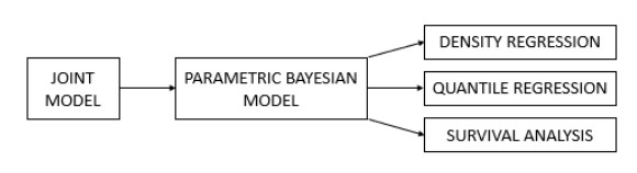
This study investigated the All Share Index (ALSI) returns and six different risk measures of the South African market for the sample period from 17 March 2000 to 17 March 2022. The risk measures analyzed were standard deviation (SD), absolute deviation (AD), lower semi absolute deviation (LSAD), lower semivariance (LSV), realized variance (RV) and the bias-adjusted realized variance (ARV). This study made an innovative contribution on a methodological and practical level, by being the first study to extend from the novel Bayesian approach by Jensen and Maheu (2018) to methods by Karabatsos (2017)—density regression, quantile regression and survival analysis. The extensions provided a full representation of the return distribution in relation to risk, through graphical analysis, producing novel insight into the risk-return topic. The most novel and innovative contribution of this study was the application of survival analysis which analyzed the "life" and "death" of the risk-return relationship. From the density regression, this study found that the chance of investors earning a superior return was substantial and that the probability of excess returns increased over time. From quantile regression, results revealed that returns have a negative relationship with the majority of the risk measures—SD, AD, LSAD and RV. However, a positive risk-return relationship was found by LSV and the ARV, with the latter having the steepest slope. Results were the most pronounced for the ARV, especially for the survival analysis. While ARV earned the highest returns, it had the shortest lifespan, which can be attributed to the volatile nature of the South African market. Thus, investors that seek short-term high-earning returns would examine ARV followed by LSV, whereas the remaining risk measures can be used for other purposes, such as diversification purposes or short selling.

References

[1]	Alles L, Murray L (2017) Asset pricing and downside risk in the Australian share market. Appl Econ 49: 4336–4350. http://dx.doi.org/10.1080/00036846.2017.1282143 doi: 10.1080/00036846.2017.1282143
[2]	Basher SA, Sadorsky P (2006) Oil price risk and emerging stock markets. Glob Financ J 17: 224–251. http://dx.doi.org/10.1016/j.gfj.2006.04.001 doi: 10.1016/j.gfj.2006.04.001
[3]	Bayes T (1763) An Essay towards Solving a Problem in the Doctrine of Chances. by the Late Rev. Mr. Bayes, F. R. S. Communicated by Mr. Price, in a Letter to John Canton, A. M. F. R. S. Phil Trans R Soc 53: 370–418. https://doi.org/10.1098/rstl.1763.0053 doi: 10.1098/rstl.1763.0053
[4]	Brooks C (2014) Introductory Econometrics for Finance. Cambridge University Press: New York.
[5]	Devore JL (2012) Probability and Statistics for Engineering and the Sciences. California Polytechnic State University: San Luis Obispo.
[6]	Emmert-Streib F, Dehmer M (2019) Introduction to Survival Analysis in Practice. Mach Learn Know Extr 1: 1013–1038. https://doi.org/10.3390/make1030058 doi: 10.3390/make1030058
[7]	Fassas AP, Siriopoulos C (2020) Implied volatility indices—A review. Q Rev Econ Financ 79: 303–329. https://doi.org/10.1016/j.qref.2020.07.004 doi: 10.1016/j.qref.2020.07.004
[8]	Floros C, Gkillas K, Konstantatos C, Tsagkanos A (2020) Realized Measures to Explain Volatility Changes over Time. J Risk Financ Manag 13: 1–19. https://doi.org/10.3390/jrfm13060125 doi: 10.3390/jrfm13060125
[9]	Gao G, Bu Z, Liu L, et al. (2019) A Survival Analysis Method for Stock Market Prediction. 2015 International Conference on Behavioral, Economic and Socio-cultural Computing (BESC), 116–122. https://doi.org/10.1109/BESC.2015.7365968 doi: 10.1109/BESC.2015.7365968
[10]	Gepp A, Kumar, K (2015) Predicting Financial Distress: A Comparison of Survival Analysis and Decision Tree Technique. Procedia Comput Sci 54: 396–404. https://doi.org/10.1016/j.procs.2015.06.046 doi: 10.1016/j.procs.2015.06.046
[11]	Griffin JE, Kalli M, Steel M (2018) Discussion of "Nonparametric Bayesian Inference in Applications": Bayesian nonparametric methods in econometrics. Stat Method Appl 27: 207–218. https://doi.org/10.1007/s10260-017-0384-0 doi: 10.1007/s10260-017-0384-0
[12]	Hansen PR, Lunde A (2006) Realized variance and market microstructure noise. J Bus Econ Stat 24: 127–161. https://doi.org/10.1198/073500106000000071 doi: 10.1198/073500106000000071
[13]	Hoque ME, Low S (2020) Industry Risk Factors and Stock Returns of Malaysian Oil and Gas Industry: A New Look with Mean Semi-Variance Asset Pricing Framework. Mathematics 8: 1–28. https://doi.org/10.3390/math8101732 doi: 10.3390/math8101732
[14]	Jensen MJ, Maheu JM (2018) Risk, Return and Volatility Feedback: A Bayesian Nonparametric Analysis. J Risk Financ Manag 11: 1–29. https://doi.org/10.3390/jrfm11030052 doi: 10.3390/jrfm11030052
[15]	Kalli M, Griffin J, Walker S (2011) Slice sampling mixture models. Stat Comput 21: 93–105. http://dx.doi.org/10.1007/s11222-009-9150-y doi: 10.1007/s11222-009-9150-y
[16]	Karabatsos G (2017) A menu-driven software package of Bayesian nonparametric (and parametric) mixed models for regression analysis and density estimation. Behav Res Methods 49: 335–362. https://doi.org/10.3758/s13428-016-0711-7 doi: 10.3758/s13428-016-0711-7
[17]	Markowitz H (1952) Portfolio selection. T J Financ 7: 77–91. https://doi.org/10.2307/2975974 doi: 10.2307/2975974
[18]	Moghaddam MD, Liu J, Serota RA (2020) Implied and realized volatility: A study of distributions and the distribution of difference. Int J Financ Econ 26: 2581–2594. https://doi.org/10.1002/ijfe.1922 doi: 10.1002/ijfe.1922
[19]	National Treasury (2021) Economic Overview. In: Chapter 2. Budget Review. Republic of South Africa. Available from: http://www.treasury.gov.za/documents/National%20Budget/2021/review/Chapter%202.pdf.
[20]	Papaspiliopoulos O (2008) A note on posterior sampling from Dirichlet mixture models. Available from: http://www2.warwick.ac.uk/fac/sci/statistics/crism/research/2008/08-20wv2.pdf.
[21]	Sehgal S, Pandey A (2018) Predicting Financial Crisis by Examining Risk-Return Relationship. Theor Econ Lett 8: 48–71. https://doi.org/10.4236/tel.2018.81003 doi: 10.4236/tel.2018.81003
[22]	Sharma S (2017) Markov Chain Monte Carlo Methods for Bayesian Data Analysis in Astronomy. Annu Rev Astron Astrophys 55: 213–259. https://doi.org/10.48550/arXiv.1706.01629 doi: 10.48550/arXiv.1706.01629
[23]	Stankovic JZ, Petrocvic E, Dencic-Mihajlov K (2020) Effects of Applying Different Risk Measures on the Optimal Portfolio Selection: The Case of the Belgrade Stock Exchange. Facta Universitatis Series: Economics and Organization 17: 17–26. https://doi.org/10.22190/FUEO191016002S doi: 10.22190/FUEO191016002S
[24]	Steyn JP, Theart L (2019) Are South African equity investors rewarded for taking on more risk? J Econ Financ Sci 12: 1–10. https://doi.org/10.4102/jef.v12i1.448 doi: 10.4102/jef.v12i1.448
[25]	Trichilli Y, Abbes MB, Masmoudi A (2020) Islamic and conventional portfolios optimization under investor sentiment states: Bayesian vs Markowitz portfolio analysis. Res Int Bus Financ 51: 1–21. https://doi.org/10.1016/j.ribaf.2019.101071 doi: 10.1016/j.ribaf.2019.101071
[26]	van Ravenzwaaij D, Cassey P, Brown SD (2018) A simple introduction to Markov Chain Monte-Carlo sampling. Psychon Bull Rev 25: 143–154. https://doi.org/10.3758/s13423-016-1015-8 doi: 10.3758/s13423-016-1015-8
[27]	Walker SG (2007) Sampling the dirichlet mixture model with slices. Commun Stat-Simul C 36: 45–54. http://dx.doi.org/10.1080/03610910601096262 doi: 10.1080/03610910601096262
[28]	Yildiz ME, Erzurumlu YO, Kurtulus B (2022) Comparative analyses of mean-variance and mean-semivariance approaches on global and local single factor market model for developed and emerging markets. Int J Emerg Mark 17: 325–350. https://doi.org/10.1108/IJOEM-01-2020-0110 doi: 10.1108/IJOEM-01-2020-0110

Reader Comments

Your name:*

Email:*
© 2022 the Author(s), licensee AIMS Press. This is an open access article distributed under the terms of the Creative Commons Attribution License (http://creativecommons.org/licenses/by/4.0)