Cannabis in the management of PTSD: a systematic review

Yasir Rehman; Amreen Saini; Sarina Huang; Emma Sood; Ravneet Gill; Sezgi Yanikomeroglu; Yasir Rehman; Amreen Saini; Sarina Huang; Emma Sood; Ravneet Gill; Sezgi Yanikomeroglu

doi:10.3934/Neuroscience.2021022

AIMS Neuroscience

2021, Volume 8, Issue 3: 414-434. doi: 10.3934/Neuroscience.2021022

Previous Article Next Article

Review

Cannabis in the management of PTSD: a systematic review

1.
Health Research Methodology, McMaster University, Hamilton, Ontario, Canada
2.
Michael DeGroote Institute of Pain and Research Center, McMaster University, Hamilton, Ontario, Canada
3.
Canadian Academy of Osteopathy, Hamilton, Ontario, Canada
4.
Faculty of Science, McMaster University, Hamilton, Ontario, Canada
5.
Faculty of Health Sciences, McMaster University, Hamilton, Ontario, Canada

Received: 17 February 2021 Accepted: 08 May 2021 Published: 13 May 2021

Introduction
Existing reviews exploring cannabis effectiveness have numerous limitations including narrow search strategies. We systematically explored cannabis effects on PTSD symptoms, quality of life (QOL), and return to work (RTW). We also investigated harm outcomes such as adverse effects and dropouts due to adverse effects, inefficacy, and all-cause dropout rates.
Methods
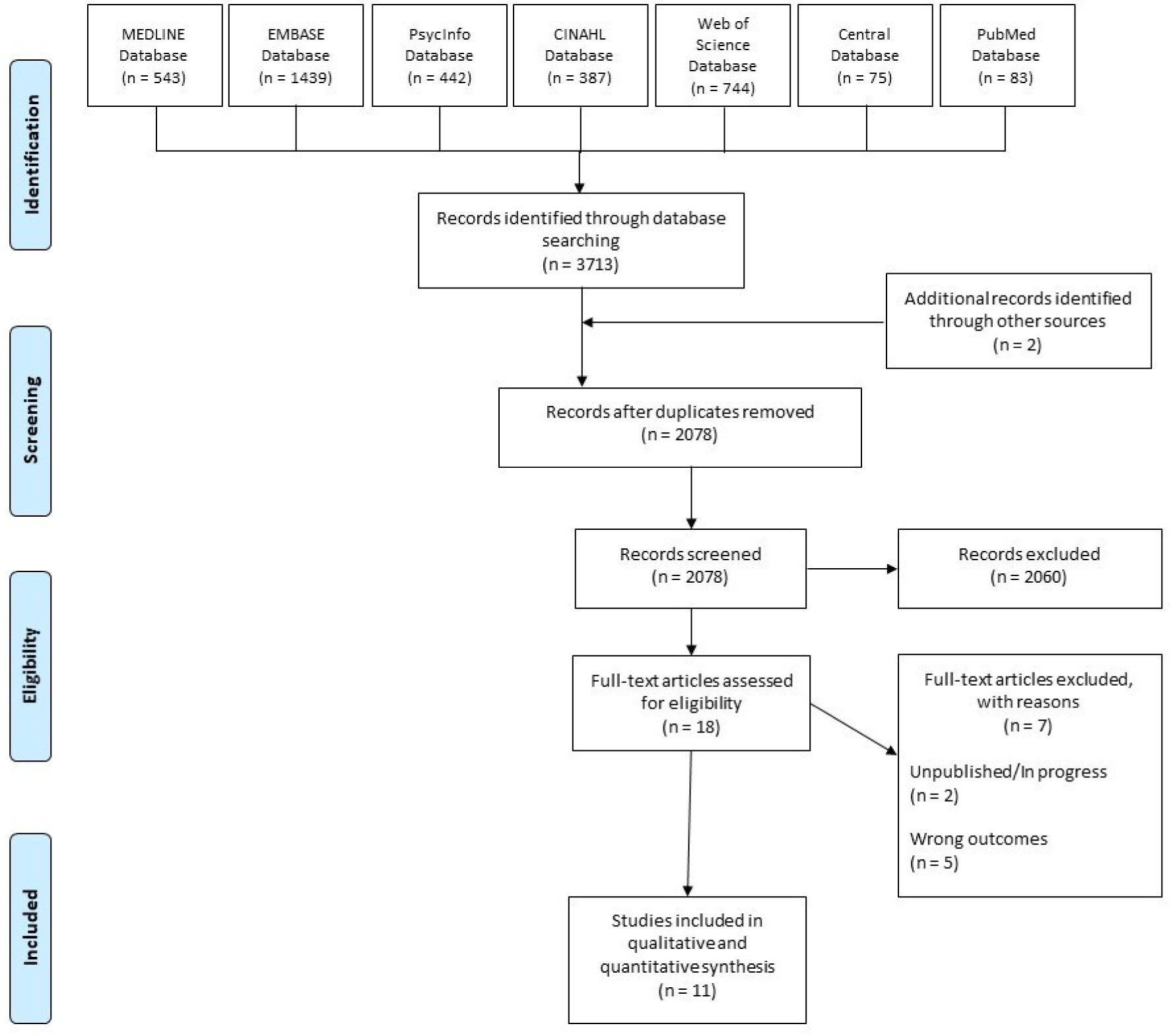
Our search in MEDLINE, EMBASE, PsycInfo, CINAHL, Web of Science, CENTRAL, and PubMed databases, yielded 1 eligible RCT and 10 observational studies (n = 4672). Risk of bias (RoB) was assessed with the Cochrane risk of bias tool and ROBINS-I.
Results
Evidence from the included studies was mainly based on non-randomized studies with no comparators. Results from unpooled, high RoB studies showed that cannabis was associated with a reduction in overall PTSD symptoms and improved QOL. Dry mouth, headaches, and psychoactive effects such as agitation and euphoria were the commonly reported adverse effects. In most studies, cannabis was well tolerated, but small proportions of patients experienced a worsening of PTSD symptoms.
Conclusion
Evidence in the current study primarily stems from low quality and high RoB observational studies. Further RCTs investigating cannabis effects on PTSD treatment should be conducted with larger sample sizes and explore a broader range of patient-important outcomes.
- PTSD,
- cannabis,
- THC,
- nabilone,
- symptoms reduction,
- functional improvement,
- systematic review,
- meta-analysis,
- cannabinoid
Citation: Yasir Rehman, Amreen Saini, Sarina Huang, Emma Sood, Ravneet Gill, Sezgi Yanikomeroglu. Cannabis in the management of PTSD: a systematic review[J]. AIMS Neuroscience, 2021, 8(3): 414-434. doi: 10.3934/Neuroscience.2021022

Related Papers:

Abstract

Introduction

Existing reviews exploring cannabis effectiveness have numerous limitations including narrow search strategies. We systematically explored cannabis effects on PTSD symptoms, quality of life (QOL), and return to work (RTW). We also investigated harm outcomes such as adverse effects and dropouts due to adverse effects, inefficacy, and all-cause dropout rates.

Methods

Our search in MEDLINE, EMBASE, PsycInfo, CINAHL, Web of Science, CENTRAL, and PubMed databases, yielded 1 eligible RCT and 10 observational studies (n = 4672). Risk of bias (RoB) was assessed with the Cochrane risk of bias tool and ROBINS-I.

Results

Evidence from the included studies was mainly based on non-randomized studies with no comparators. Results from unpooled, high RoB studies showed that cannabis was associated with a reduction in overall PTSD symptoms and improved QOL. Dry mouth, headaches, and psychoactive effects such as agitation and euphoria were the commonly reported adverse effects. In most studies, cannabis was well tolerated, but small proportions of patients experienced a worsening of PTSD symptoms.

Conclusion

Evidence in the current study primarily stems from low quality and high RoB observational studies. Further RCTs investigating cannabis effects on PTSD treatment should be conducted with larger sample sizes and explore a broader range of patient-important outcomes.

Conflict of interest

The authors declare no conflict of interest.

References

[1]	Stein DJ, McLaughlin KA, Koenen KC, et al. (2014) DSM-5 and ICD-11 definitions of posttraumatic stress disorder: investigating “narrow” and “broad” approaches. Depress Anxiety 31: 494-505. doi: 10.1002/da.22279
[2]	Pai A, Suris AM, North CS (2017) Posttraumatic Stress Disorder in the DSM-5: Controversy, Change, and Conceptual Considerations. Behav Sci (Basel) 7: 7. doi: 10.3390/bs7010007
[3]	Richardson LK, Frueh BC, Acierno R (2010) Prevalence estimates of combat-related post-traumatic stress disorder: critical review. Aust N Z J Psychiatry 44: 4-19. doi: 10.3109/00048670903393597
[4]	Rehman Y, Sadeghirad B, Guyatt GH, et al. (2019) Management of post-traumatic stress disorder: A protocol for a multiple treatment comparison meta-analysis of randomized controlled trials. Medicine 98: e17064. doi: 10.1097/MD.0000000000017064
[5]	Acheson DT, Gresack JE, Risbrough VB (2012) Hippocampal dysfunction effects on context memory: possible etiology for posttraumatic stress disorder. Neuropharmacology 62: 674-685. doi: 10.1016/j.neuropharm.2011.04.029
[6]	Kar N (2011) Cognitive behavioral therapy for the treatment of post-traumatic stress disorder: a review. Neuropsychiatr Dis Treat 7: 167-181. doi: 10.2147/NDT.S10389
[7]	Zoellner LA, Feeny NC, Bittinger JN, et al. (2011) Teaching Trauma-Focused Exposure Therapy for PTSD: Critical Clinical Lessons for Novice Exposure Therapists. Psychol Trauma 3: 300-308. doi: 10.1037/a0024642
[8]	Rothbaum BO, Schwartz AC (2002) Exposure therapy for posttraumatic stress disorder. Am J Psychother 56: 59-75. doi: 10.1176/appi.psychotherapy.2002.56.1.59
[9]	Chiba T, Kanazawa T, Koizumi A, et al. (2019) Current Status of Neurofeedback for Post-traumatic Stress Disorder: A Systematic Review and the Possibility of Decoded Neurofeedback. Front Hum Neurosci 13: 233. doi: 10.3389/fnhum.2019.00233
[10]	Zepeda Méndez M, Nijdam MJ, Ter Heide FJJ, et al. (2018) A five-day inpatient EMDR treatment programme for PTSD: pilot study. Eur J Psychotraumatol 9: 1425575. doi: 10.1080/20008198.2018.1425575
[11]	Stein DJ, Ipser JC, Seedat S (2006) Pharmacotherapy for post traumatic stress disorder (PTSD). Cochrane Database Syst Rev 2006: CD002795.
[12]	Ravindran LN, Stein MB (2009) Pharmacotherapy of PTSD: premises, principles, and priorities. Brain Res 1293: 24-39. doi: 10.1016/j.brainres.2009.03.037
[13]	Ipser JC, Stein DJ (2012) Evidence-based pharmacotherapy of post-traumatic stress disorder (PTSD). Int J Neuropsychopharmacol 15: 825-840. doi: 10.1017/S1461145711001209
[14]	Krumm BA (2016) Cannabis for posttraumatic stress disorder: A neurobiological approach to treatment. Nurse Pract 41: 50-54. doi: 10.1097/01.NPR.0000434091.34348.3c
[15]	Téllez-Zenteno JF, Hernández-Ronquillo L (2020) Medical Cannabis as a Treatment for Patients With Epilepsy, Sleep Disorders, and Posttraumatic Stress Disorder. J Clin Neurophysiol 37: 1. doi: 10.1097/WNP.0000000000000650
[16]	Passie T, Emrich HM, Karst M, et al. (2012) Mitigation of post-traumatic stress symptoms by Cannabis resin: A review of the clinical and neurobiological evidence. Drug Test Anal 4: 649-659. doi: 10.1002/dta.1377
[17]	Bremner JD (2006) Traumatic stress: effects on the brain. Dialogues Clin Neurosci 8: 445-461. doi: 10.31887/DCNS.2006.8.4/jbremner
[18]	Kinlein SA, Wilson CD, Karatsoreos IN (2015) Dysregulated hypothalamic-pituitary-adrenal axis function contributes to altered endocrine and neurobehavioral responses to acute stress. Front Psychiatry 6: 31. doi: 10.3389/fpsyt.2015.00031
[19]	Sherin JE, Nemeroff CB (2011) Post-traumatic stress disorder: the neurobiological impact of psychological trauma. Dialogues Clin Neurosci 13: 263-278. doi: 10.31887/DCNS.2011.13.2/jsherin
[20]	Zou S, Kumar U (2018) Cannabinoid Receptors and the Endocannabinoid System: Signaling and Function in the Central Nervous System. Int J Mol Sci 19: 833. doi: 10.3390/ijms19030833
[21]	Hindocha C, Cousijn J, Rall M, et al. (2020) The Effectiveness of Cannabinoids in the Treatment of Posttraumatic Stress Disorder (PTSD): A Systematic Review. J Dual Diagn 16: 120-139. doi: 10.1080/15504263.2019.1652380
[22]	O'Neil ME, Nugent SM, Morasco BJ, et al. (2017) Benefits and Harms of Plant-Based Cannabis for Posttraumatic Stress Disorder: A Systematic Review. Ann Intern Med 167: 332-340. doi: 10.7326/M17-0477
[23]	Orsolini L, Chiappini S, Volpe U, et al. (2019) Use of Medicinal Cannabis and Synthetic Cannabinoids in Post-Traumatic Stress Disorder (PTSD): A Systematic Review. Medicina (Kaunas) 55: 525. doi: 10.3390/medicina55090525
[24]	Shishko I, Oliveira R, Moore TA, et al. (2018) A review of medical marijuana for the treatment of posttraumatic stress disorder: Real symptom re-leaf or just high hopes? Ment Health Clin 8: 86-94. doi: 10.9740/mhc.2018.03.086
[25]	Yarnell S (2015) The Use of Medicinal Marijuana for Posttraumatic Stress Disorder: A Review of the Current Literature. Prim Care Companion CNS Disord 17.
[26]	Carnes D, Mullinger B, Underwood M (2010) Defining adverse events in manual therapies: a modified Delphi consensus study. Man Ther 15: 2-6. doi: 10.1016/j.math.2009.02.003
[27]	Carlesso LC, Cairney J, Dolovich L, et al. (2011) Defining adverse events in manual therapy: an exploratory qualitative analysis of the patient perspective. Man Ther 16: 440-446. doi: 10.1016/j.math.2011.02.001
[28]	Liberati A, Altman DG, Tetzlaff J, et al. (2009) The PRISMA statement for reporting systematic reviews and meta-analyses of studies that evaluate healthcare interventions: explanation and elaboration. BMJ 339: b2700. doi: 10.1136/bmj.b2700
[29]	Zorzela L, Loke YK, Ioannidis JP, et al. (2016) PRISMA harms checklist: improving harms reporting in systematic reviews. BMJ 352: i157. doi: 10.1136/bmj.i157
[30]	Zorzela L, Golder S, Liu YL, et al. (2014) Quality of reporting in systematic reviews of adverse events: systematic review. BMJ 348: f7668. doi: 10.1136/bmj.f7668
[31]	Reeves BC, Higgins JPT, Higgins JPT, et al. (2019) Including non-randomized studies on intervention effects. Cochrane Handbook for Systematic Reviews of Interventions version 60 Available from: www.training.cochrane.org/handbook.
[32]	Higgins JPT, Altman DG, JAC S (2011) Assessing risk of bias in included studies. Cochrane Handbook for Systematic Reviews of Interventions The Cochrane Collaboration.
[33]	Sterne JA, Hernan MA, Reeves BC, et al. (2016) ROBINS-I: a tool for assessing risk of bias in non-randomised studies of interventions. BMJ 355: i4919. doi: 10.1136/bmj.i4919
[34]	Jetly R, Heber A, Fraser G, et al. (2015) The efficacy of nabilone, a synthetic cannabinoid, in the treatment of PTSD-associated nightmares: A preliminary randomized, double-blind, placebo-controlled cross-over design study. Psychoneuroendocrinology 51: 585-588. doi: 10.1016/j.psyneuen.2014.11.002
[35]	Chan S, Wolt A, Zhang L, et al. (2017) Medical cannabis use for patients with post-traumatic stress disorder (PTSD). J Pain Manage 10.
[36]	Drost L, Wan B, Chan S, et al. (2017) Efficacy of different varieties of medical cannabis in relieving symptoms in post-traumatic stress disorder (PTSD) patients. J Pain Manage 10.
[37]	Smith P, Chan S, Blake A, et al. (2017) Medical cannabis use in military and police veterans diagnosed with post-traumatic stress disorder (PTSD). J Pain Manage 10: 397-405.
[38]	Elms L, Shannon S, Hughes S, et al. (2019) Cannabidiol in the Treatment of Post-Traumatic Stress Disorder: A Case Series. J Altern Complement Med 25: 392-397. doi: 10.1089/acm.2018.0437
[39]	Cameron C, Watson D, Robinson J (2014) Use of a synthetic cannabinoid in a correctional population for posttraumatic stress disorder-related insomnia and nightmares, chronic pain, harm reduction, and other indications: a retrospective evaluation. J Clin Psychopharmacol 34: 559-564. doi: 10.1097/JCP.0000000000000180
[40]	Greer GR, Grob CS, Halberstadt AL (2014) PTSD symptom reports of patients evaluated for the New Mexico Medical Cannabis Program. J Psychoactive Drugs 46: 73-77. doi: 10.1080/02791072.2013.873843
[41]	Johnson MJ, Pierce JD, Mavandadi S, et al. (2016) Mental health symptom severity in cannabis using and non-using Veterans with probable PTSD. J Affect Disord 190: 439-442. doi: 10.1016/j.jad.2015.10.048
[42]	Roitman P, Mechoulam R, Cooper-Kazaz R, et al. (2014) Preliminary, open-label, pilot study of add-on oral Delta9-tetrahydrocannabinol in chronic post-traumatic stress disorder. Clin Drug Investig 34: 587-591. doi: 10.1007/s40261-014-0212-3
[43]	Wilkinson ST, Stefanovics E, Rosenheck RA (2015) Marijuana use is associated with worse outcomes in symptom severity and violent behavior in patients with posttraumatic stress disorder. J Clin Psychiatry 76: 1174-1180. doi: 10.4088/JCP.14m09475
[44]	Ruglass LM, Shevorykin A, Radoncic V, et al. (2017) Impact of Cannabis Use on Treatment Outcomes among Adults Receiving Cognitive-Behavioral Treatment for PTSD and Substance Use Disorders. J Clin Med 6: 14. doi: 10.3390/jcm6020014
[45]	Dagan Y, Yager J (2020) Cannabis and Complex Posttraumatic Stress Disorder: A Narrative Review With Considerations of Benefits and Harms. J Nerv Ment Dis 208: 619-627. doi: 10.1097/NMD.0000000000001172
[46]	McIntosh HM, Woolacott NF, Bagnall AM (2004) Assessing harmful effects in systematic reviews. BMC Med Res Methodol 4: 19. doi: 10.1186/1471-2288-4-19
[47]	Ernst E, Pittler MH (2001) Assessment of therapeutic safety in systematic reviews: literature review. BMJ 323: 546. doi: 10.1136/bmj.323.7312.546
[48]	LaFrance EM, Glodosky NC, Bonn-Miller M, et al. (2020) Short and Long-Term Effects of Cannabis on Symptoms of Post-Traumatic Stress Disorder. J Affec Disord 274: 298-304. doi: 10.1016/j.jad.2020.05.132
[49]	Khan R, Naveed S, Mian N, et al. (2020) The therapeutic role of Cannabidiol in mental health: a systematic review. J Cannabis Res 2: 2. doi: 10.1186/s42238-019-0012-y
[50]	Shalev A, Liberzon I, Marmar C (2017) Post-Traumatic Stress Disorder. N Engl J Med 376: 2459-2469. doi: 10.1056/NEJMra1612499
[51]	Hill MN, Campolongo P, et al. (2018) Integrating Endocannabinoid Signaling and Cannabinoids into the Biology and Treatment of Posttraumatic Stress Disorder. Neuropsychopharmacology 43: 80-102. doi: 10.1038/npp.2017.162
[52]	Kimerling R, Allen MC, Duncan LE (2018) Chromosomes to Social Contexts: Sex and Gender Differences in PTSD. Curr Psychiatry Rep 20: 114. doi: 10.1007/s11920-018-0981-0
[53]	Abizaid A, Merali Z, Anisman H (2019) Cannabis: A potential efficacious intervention for PTSD or simply snake oil? J Psychiatry Neurosci 44: 75-78. doi: 10.1503/jpn.190021
[54]	Campbell RL, Germain A (2016) Nightmares and Posttraumatic Stress Disorder (PTSD). Curr Sleep Med Rep 2: 74-80. doi: 10.1007/s40675-016-0037-0
[55]	Schnurr PP, Lunney CA (2012) Work-related outcomes among female veterans and service members after treatment of posttraumatic stress disorder. Psychiatr Serv 63: 1072-1079. doi: 10.1176/appi.ps.201100415
[56]	Schnurr PP, Lunney CA (2016) SYMPTOM BENCHMARKS OF IMPROVED QUALITY OF LIFE IN PTSD. Depress Anxiety 33: 247-255. doi: 10.1002/da.22477
[57]	Madden SP, Einhorn PM (2018) Cannabis-Induced Depersonalization-Derealization Disorder. AJ P-RJ 13: 3-6.
[58]	Tull MT, McDermott MJ, Gratz KL (2016) Marijuana dependence moderates the effect of posttraumatic stress disorder on trauma cue reactivity in substance dependent patients. Drug Alcohol Depend 159: 219-226. doi: 10.1016/j.drugalcdep.2015.12.014
[59]	Boden MT, Babson KA, Vujanovic AA, et al. (2013) Posttraumatic stress disorder and cannabis use characteristics among military veterans with cannabis dependence. Am J Addict 22: 277-284. doi: 10.1111/j.1521-0391.2012.12018.x
[60]	Kansagara D, O'Neil M, Nugent S, et al. (2017) Benefits and Harms of Cannabis in Chronic Pain or Post-traumatic Stress Disorder: A Systematic Review. Dep Veterans Aff .
[61]	Bonnet U, Preuss UW (2017) The cannabis withdrawal syndrome: current insights. Subst Abuse Rehabil 8: 9-37. doi: 10.2147/SAR.S109576
[62]	Black N, Stockings E, Campbell G, et al. (2019) Cannabinoids for the treatment of mental disorders and symptoms of mental disorders: a systematic review and meta-analysis. Lancet Psychiatry 6: 995-1010. doi: 10.1016/S2215-0366(19)30401-8
[63]	Foa EB, Meadows EA (1997) Psychosocial treatments for posttraumatic stress disorder: A critical review. Annu Rev Psychol 48: 449-480. doi: 10.1146/annurev.psych.48.1.449

Reader Comments

your name:*

Email:*
© 2021 the Author(s), licensee AIMS Press. This is an open access article distributed under the terms of the Creative Commons Attribution License (http://creativecommons.org/licenses/by/4.0)