The role of tetrahydrocannabivarin (THCV) in metabolic disorders: A promising cannabinoid for diabetes and weight management

Scott Mendoza; Scott Mendoza

doi:10.3934/Neuroscience.2025003

AIMS Neuroscience

2025, Volume 12, Issue 1: 32-43. doi: 10.3934/Neuroscience.2025003

Previous Article Next Article

Mini review Special Issues

The role of tetrahydrocannabivarin (THCV) in metabolic disorders: A promising cannabinoid for diabetes and weight management

Scott Mendoza ^,

Department of Biomedical Laboratory Science, Namseoul University, Cheonan 31020, Republic of Korea

Received: 21 December 2024 Revised: 19 February 2025 Accepted: 05 March 2025 Published: 12 March 2025

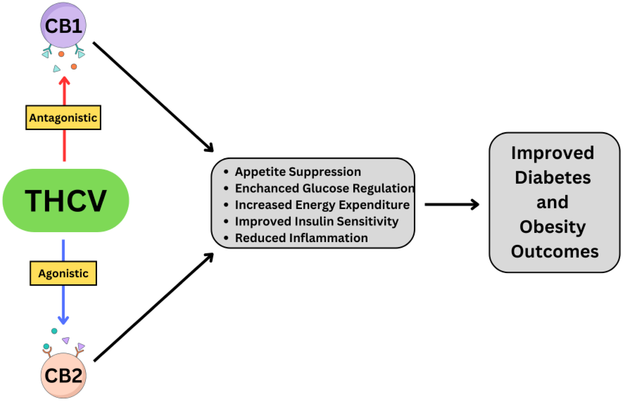
Disorders of the metabolism, including obesity and type 2 diabetes, represent significant global health challenges due to their rising prevalence and associated complications. Despite existing therapeutic strategies, including lifestyle interventions, pharmacological treatments, and surgical options, limitations such as poor adherence, side effects, and accessibility issues call attention to the need for novel solutions. Tetrahydrocannabivarin (THCV), a non-psychoactive cannabinoid derived from Cannabis sativa, has emerged as a promising agent to manage metabolic disorders. Unlike tetrahydrocannabinol (THC), THCV exhibits an antagonistic function on the CB1 receptor and a partial agonist function on the CB2 receptor, thus enabling appetite suppression, enhanced glucose regulation, and increased energy expenditure. Preclinical studies demonstrated that THCV improves insulin sensitivity, promotes glucose uptake, and restores insulin signaling in metabolic tissues. Additionally, THCV reduces lipid accumulation and improves the mitochondrial activity in adipocytes and hepatocytes, shown through both cell-based and animal research. Animal models further revealed THCV's potential to suppress appetite, prevent hepatosteatosis, and improve metabolic homeostasis. Preliminary human trials support these findings, thereby showing that THCV may modulate appetite and glycemic control, though larger-scale studies are necessary to confirm its clinical efficacy and safety. THCV's unique pharmacological profile positions it as a possible therapeutic candidate to address the multifaceted challenges of obesity and diabetes. Continued research should concentrate on optimizing formulations, undertaking well-designed clinical studies, and addressing regulatory hurdles to unlock its full potential.
- tetrahydrocannabivarin (THCV),
- metabolic disorders,
- obesity management,
- type 2 diabetes,
- cannabinoids,
- appetite suppression,
- glucose regulation,
- endocannabinoid system,
- insulin sensitivity
Citation: Scott Mendoza. The role of tetrahydrocannabivarin (THCV) in metabolic disorders: A promising cannabinoid for diabetes and weight management[J]. AIMS Neuroscience, 2025, 12(1): 32-43. doi: 10.3934/Neuroscience.2025003

Related Papers:

Abstract

Disorders of the metabolism, including obesity and type 2 diabetes, represent significant global health challenges due to their rising prevalence and associated complications. Despite existing therapeutic strategies, including lifestyle interventions, pharmacological treatments, and surgical options, limitations such as poor adherence, side effects, and accessibility issues call attention to the need for novel solutions. Tetrahydrocannabivarin (THCV), a non-psychoactive cannabinoid derived from Cannabis sativa, has emerged as a promising agent to manage metabolic disorders. Unlike tetrahydrocannabinol (THC), THCV exhibits an antagonistic function on the CB1 receptor and a partial agonist function on the CB2 receptor, thus enabling appetite suppression, enhanced glucose regulation, and increased energy expenditure. Preclinical studies demonstrated that THCV improves insulin sensitivity, promotes glucose uptake, and restores insulin signaling in metabolic tissues. Additionally, THCV reduces lipid accumulation and improves the mitochondrial activity in adipocytes and hepatocytes, shown through both cell-based and animal research. Animal models further revealed THCV's potential to suppress appetite, prevent hepatosteatosis, and improve metabolic homeostasis. Preliminary human trials support these findings, thereby showing that THCV may modulate appetite and glycemic control, though larger-scale studies are necessary to confirm its clinical efficacy and safety. THCV's unique pharmacological profile positions it as a possible therapeutic candidate to address the multifaceted challenges of obesity and diabetes. Continued research should concentrate on optimizing formulations, undertaking well-designed clinical studies, and addressing regulatory hurdles to unlock its full potential.

Acknowledgments

Funding for this paper was provided by Namseoul University.

Conflict of interest

The author of this paper has declared no conflicts of interest.

References

[1]	Sun H, Saeedi P, Karuranga S, et al. (2022) IDF Diabetes Atlas: Global, regional and country-level diabetes prevalence estimates for 2021 and projections for 2045. Diabetes Res Clin Pract 183: 109119. https://doi.org/10.1016/j.diabres.2021.109119
[2]	Malik VS, Willet WC, Hu FB (2020) Nearly a decade on—trends, risk factors and policy implications in global obesity. Nat Rev Endocrinol 16: 615-616. https://doi.org/10.1038/s41574-020-00411-y
[3]	Williams DM, Nawaz A, Evans M (2020) Drug therapy in obesity: a review of current and emerging treatments. Diabetes Ther 11: 1199-1216. https://doi.org/10.1007/s13300-020-00816-y
[4]	Sims EK, Carr AL J, Oram RA, et al. (2021) 100 years of insulin: celebrating the past, present and future of diabetes therapy. Nat Med 27: 1154-1164. https://doi.org/10.1038/s41591-021-01418-2
[5]	Arterburn DE, Telem DA, Kushner RF, et al. (2020) Benefits and risks of bariatric surgery in adults: a review. JAMA 324: 879-887. https://doi.org/10.1001/jama.2020.12567
[6]	Boonpattharatthiti K, Saensook T, Neelapaijit N, et al. (2024) The prevalence of adherence to insulin therapy in patients with diabetes: A systematic review and meta-analysis. Res Social Adm Pharm 20: 255-295. https://doi.org/10.1016/j.sapharm.2023.11.009
[7]	Tak YJ, Lee SY (2021) Long-term efficacy and safety of anti-obesity treatment: where do we stand?. Curr Obes Rep 10: 14-30. https://doi.org/10.1007/s13679-020-00422-w
[8]	Charytoniuk T, Zywno H, Berk K, et al. (2022) The endocannabinoid system and physical activity—a robust duo in the novel therapeutic approach against metabolic disorders. Int J Mol Sci 23: 3083. https://doi.org/10.3390/ijms23063083
[9]	Ghasemi-Gojani E, Kovalchuk I, Kovalchuk O (2022) Cannabinoids and terpenes for diabetes mellitus and its complications: From mechanisms to new therapies. Trends Endocrinol Metab 33: 828-849. https://doi.org/10.1016/j.tem.2022.08.003
[10]	Cavalheiro EKFF, Costa AB, Salla DH, et al. (2022) Cannabis sativa as a treatment for obesity: From anti-inflammatory indirect support to a promising metabolic re-establishment target. Cannabis Cannabinoid Res 7: 135-151. https://doi.org/10.1089/can.2021.0016
[11]	Murray CH, Gannon BM, Winsauer PJ, et al. (2024) The development of cannabinoids as therapeutic agents in the United States. Pharmacol Rev 76: 915-955. https://doi.org/10.1124/pharmrev.123.001121
[12]	Abioye A, Ayodele O, Marinkovic A, et al. (2020) Δ9-Tetrahydrocannabivarin (THCV): a commentary on potential therapeutic benefit for the management of obesity and diabetes. J Cannabis Res 2: 1-6. https://doi.org/10.1186/s42238-020-0016-7
[13]	Peters EN, MacNair L, Harrison A, et al. (2023) A Two-Phase, Dose-Ranging, Placebo-Controlled Study of the Safety and Preliminary Test of Acute Effects of Oral Δ8-Tetrahydrocannabivarin in Healthy Participants. Cannabis Cannabinoid Res 8: S71-S82. https://doi.org/10.1089/can.2023.0038
[14]	Haghdoost M, Peters EN, Roberts M, et al. (2025) Tetrahydrocannabivarin is Not Tetrahydrocannabinol. Cannabis Cannabinoid Res 10: 1-5. https://doi.org/10.1089/can.2024.0051
[15]	Kowalczuk A, Marycz K, Kornicka J, et al. (2023) Tetrahydrocannabivarin (THCV) Protects Adipose-Derived Mesenchymal Stem Cells (ASC) against Endoplasmic Reticulum Stress Development and Reduces Inflammation during Adipogenesis. Int J Mol Sci 24: 7120. https://doi.org/10.3390/ijms24087120
[16]	Svízenská I, Dubový P, Sulcová A (2008) Cannabinoid receptors 1 and 2 (CB1 and CB2), their distribution, ligands and functional involvement in nervous system structures--a short review. Pharmacol Biochem Behav 90: 501-511. https://doi.org/10.1016/j.pbb.2008.05.010
[17]	Kurtov M, Rubinić I, Likić R (2024) The endocannabinoid system in appetite regulation and treatment of obesity. Pharmacol Res Perspect 12: e70009. https://doi.org/10.1002/prp2.70009
[18]	Rohbeck E, Eckel J, Romacho T (2021) Cannabinoid Receptors in Metabolic Regulation and Diabetes. Physiology (Bethesda) 36: 102-113. https://doi.org/10.1152/physiol.00029.2020
[19]	Englund A, Atakan Z, Kralj A, et al. (2016) The effect of five day dosing with THCV on THC-induced cognitive, psychological and physiological effects in healthy male human volunteers: A placebo-controlled, double-blind, crossover pilot trial. J Psychopharmacol 30: 140-151. https://doi.org/10.1177/0269881115615104
[20]	Mackie K, Ross RA (2008) CB2 cannabinoid receptors: new vistas. Br J Pharmacol 153: 177-178. https://doi.org/10.1038/sj.bjp.0707617
[21]	Bátkai S, Mukhopadhyay P, Horváth B, et al. (2012) Δ8-Tetrahydrocannabivarin prevents hepatic ischaemia/reperfusion injury by decreasing oxidative stress and inflammatory responses through cannabinoid CB2 receptors. Br J Pharmacol 165: 2450-2461. https://doi.org/10.1111/j.1476-5381.2011.01410.x
[22]	Wargent ET, Zaibi MS, Silvestri C, et al. (2013) The cannabinoid Δ(9)-tetrahydrocannabivarin (THCV) ameliorates insulin sensitivity in two mouse models of obesity. Nutr Diabetes 3: e68. https://doi.org/10.1038/nutd.2013.9
[23]	Wargent ET, Kepczynska M, Zaibi MS, et al. (2020) High fat-fed GPR55 null mice display impaired glucose tolerance without concomitant changes in energy balance or insulin sensitivity but are less responsive to the effects of the cannabinoids rimonabant or Δ(9)-tetrahydrocannabivarin on weight gain. PeerJ 8: e9811. https://doi.org/10.7717/peerj.9811
[24]	Jadoon KA, Ratcliffe SH, Barrett DA, et al. (2016) Efficacy and Safety of Cannabidiol and Tetrahydrocannabivarin on Glycemic and Lipid Parameters in Patients With Type 2 Diabetes: A Randomized, Double-Blind, Placebo-Controlled, Parallel Group Pilot Study. Diabetes Care 39: 1777-1786. https://doi.org/10.2337/dc16-0650
[25]	Riedel G, Fadda P, McKillop-Smith S, et al. (2009) Synthetic and plant-derived cannabinoid receptor antagonists show hypophagic properties in fasted and non-fasted mice. Br J Pharmacol 156: 1154-1166. https://doi.org/10.1111/j.1476-5381.2008.00107.x
[26]	Silvestri C, Paris D, Martella A, et al. (2015) Two non-psychoactive cannabinoids reduce intracellular lipid levels and inhibit hepatosteatosis. J Hepatol 62: 1382-1390. https://doi.org/10.1016/j.jhep.2015.01.001
[27]	Tudge L, Williams C, Cowen PJ, et al. (2014) Neural effects of cannabinoid CB1 neutral antagonist tetrahydrocannabivarin on food reward and aversion in healthy volunteers. Int J Neuropsychopharmacol 18: pyu094. https://doi.org/10.1093/ijnp/pyu094
[28]	Stella N (2023) THC and CBD: Similarities and differences between siblings. Neuron 111: 302-327. https://doi.org/10.1016/j.neuron.2022.12.022
[29]	Farrimond JA, Mercier MS, Whalley BJ, et al. (2011) Cannabis sativa and the endogenous cannabinoid system: therapeutic potential for appetite regulation. Phytother Res 25: 170-188. https://doi.org/10.1002/ptr.3375
[30]	Naef M, Curatolo M, Petersen-Felix S, et al. (2003) The analgesic effect of oral delta-9-tetrahydrocannabinol (THC), morphine, and a THC-morphine combination in healthy subjects under experimental pain conditions. Pain 105: 79-88. https://doi.org/10.1016/S0304-3959(03)00163-5
[31]	Peng J, Fan M, An C, et al. (2022) A narrative review of molecular mechanism and therapeutic effect of cannabidiol (CBD). Basic Clin Pharmacol Toxicol 130: 439-456. https://doi.org/10.1111/bcpt.13710
[32]	Luo X, Reiter MA, d'Espaux L, et al. (2019) Complete biosynthesis of cannabinoids and their unnatural analogues in yeast. Nature 567: 123-126. https://doi.org/10.1038/s41586-019-0978-9
[33]	Bolaños-Martínez OC, Malla A, Rosales-Mendoza S, et al. (2023) Harnessing the advances of genetic engineering in microalgae for the production of cannabinoids. Crit Rev Biotechnol 43: 823-834. https://doi.org/10.1080/07388551.2022.2071672
[34]	Deiana S, Watanabe A, Yamasaki Y, et al. (2012) Plasma and brain pharmacokinetic profile of cannabidiol (CBD), cannabidivarine (CBDV), Δ⁹-tetrahydrocannabivarin (THCV) and cannabigerol (CBG) in rats and mice following oral and intraperitoneal administration and CBD action on obsessive-compulsive behaviour. Psychopharmacology (Berl) 219: 859-873. https://doi.org/10.1007/s00213-011-2415-0
[35]	Mead A (2019) Legal and Regulatory Issues Governing Cannabis and Cannabis-Derived Products in the United States. Front Plant Sci 10: 697. https://doi.org/10.3389/fpls.2019.00697
[36]	Senatore F (2023) Good Clinical Practice in Clinical Trials, Substantial Evidence of Efficacy, and Interpretation of the Evidence. The Quintessence of Basic and Clinical Research and Scientific Publishing . Singapore: Springer Nature Singapore 373-385. https://doi.org/10.1007/978-981-99-1284-1_23
[37]	Loganathan P, Gajendran M, Goyal H (2024) A Comprehensive Review and Update on Cannabis Hyperemesis Syndrome. Pharmaceuticals (Basel) 17: 1549. https://doi.org/10.3390/ph17111549
[38]	Groening JM, Denton E, Parvaiz R, et al. (2024) A systematic evidence map of the association between cannabis use and psychosis-related outcomes across the psychosis continuum: An umbrella review of systematic reviews and meta-analyses. Psychiatry Res 331: 115626. https://doi.org/10.1016/j.psychres.2023.115626
[39]	Cheng Z, Zheng L, Almeida FA (2018) Epigenetic reprogramming in metabolic disorders: nutritional factors and beyond. J Nutr Biochem 54: 1-10. https://doi.org/10.1016/j.jnutbio.2017.10.004

Reader Comments

Your name:*

Email:*
© 2025 the Author(s), licensee AIMS Press. This is an open access article distributed under the terms of the Creative Commons Attribution License (http://creativecommons.org/licenses/by/4.0)