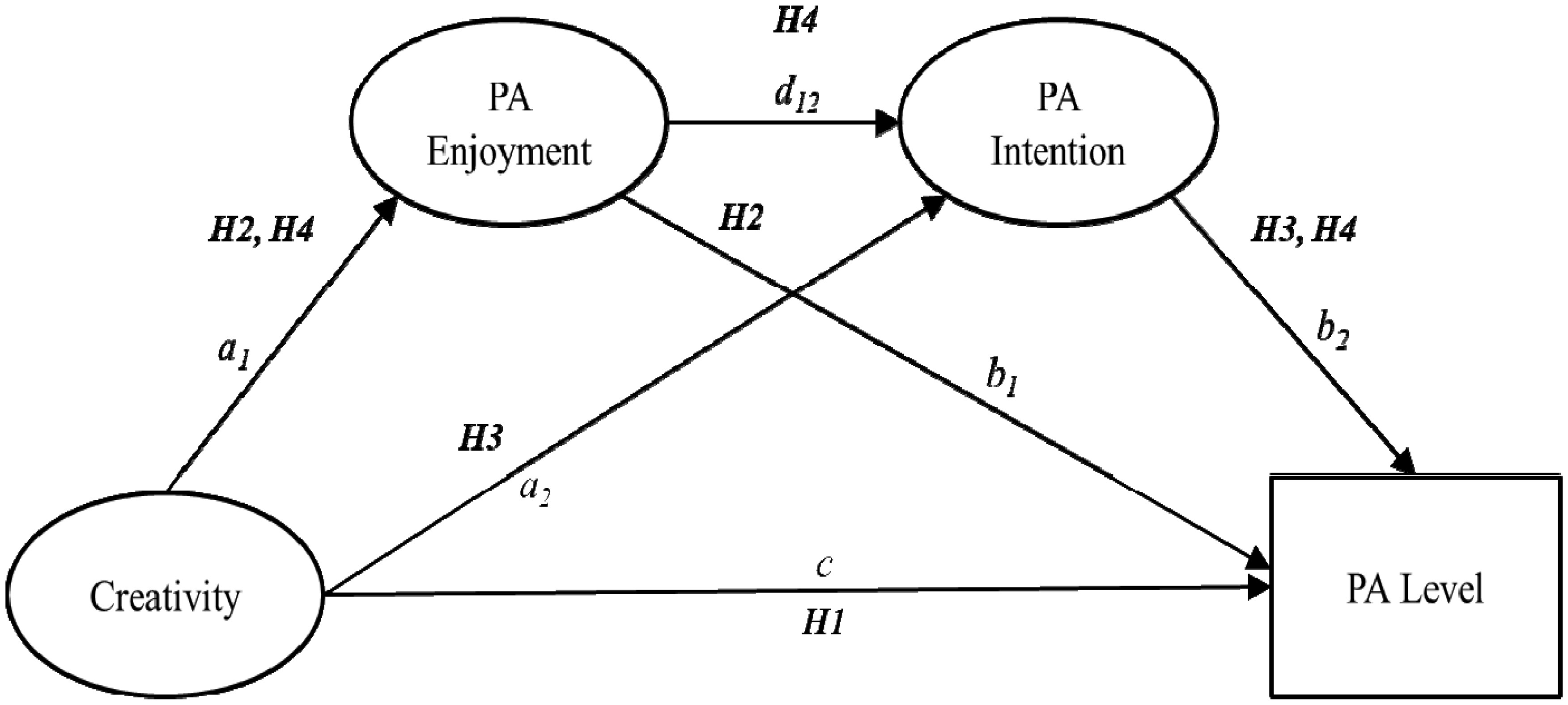
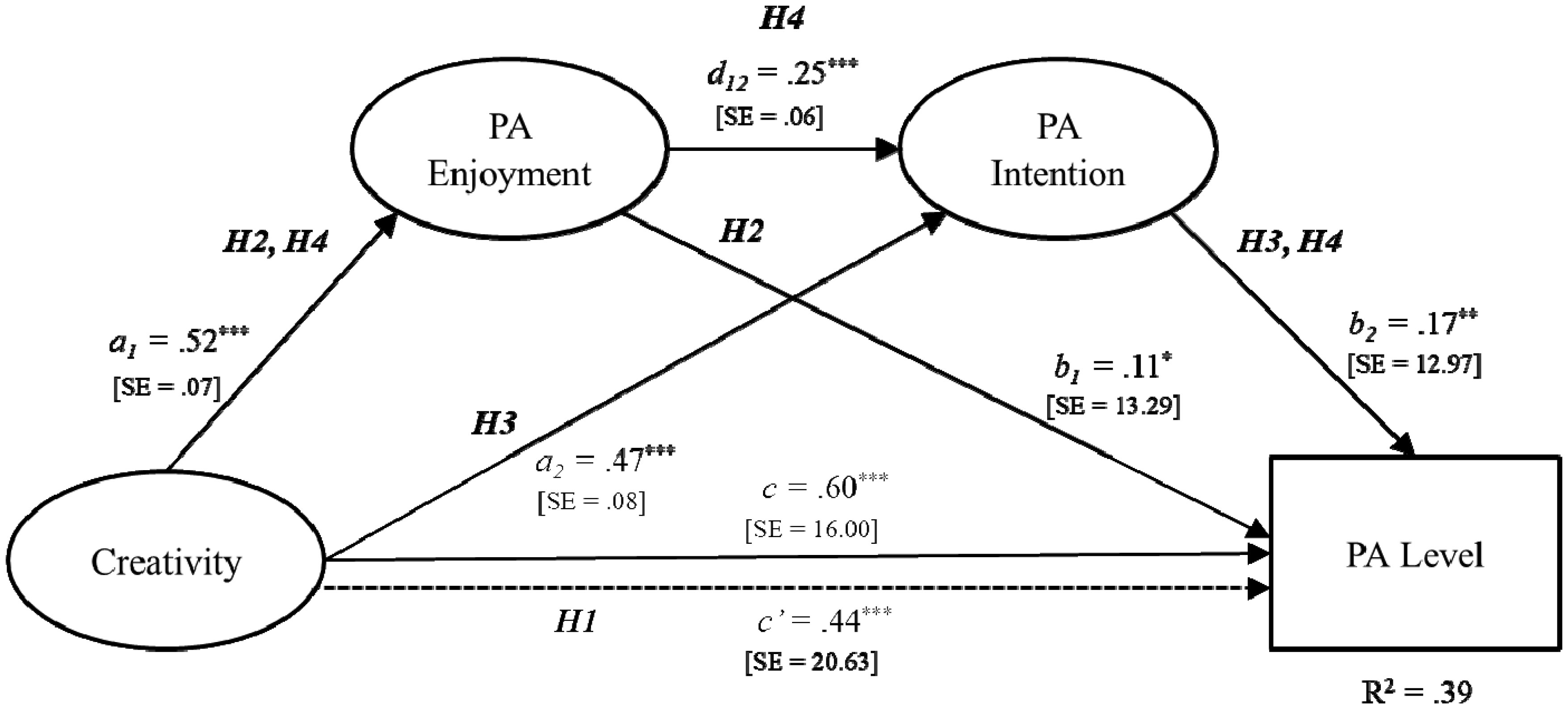
The purpose of the present study was to examine a serial-multiple mediation of physical activity (PA) enjoyment and PA intention in the relationship between creativity and PA level (i.e., moderate-to-vigorous PA). A total of 298 undergraduate and graduate students completed a self-reported questionnaire evaluating creativity, PA enjoyment, PA intention, and PA level. Data analysis was conducted using descriptive statistics, Pearson correlation coefficient, ordinary least-squares regression analysis, and bootstrap methodology. Based on the research findings, both PA enjoyment (β = 0.06; 95% CI [0.003, 0.12]) and PA intention (β = 0.08; 95% CI [0.03, 0.13]) were found to be a mediator of the relationship between creativity and PA level, respectively. Moreover, the serial-multiple mediation of PA enjoyment and PA intention in the relationship between creativity and PA level was statistically significant (β = 0.02; 95% CI [0.01, 0.04]). These findings underscore the importance of shaping both cognitive and affective functions for PA promotion and provide additional support for a neurocognitive affect-related model in the PA domain. In order to guide best practices for PA promotion programs aimed at positively influencing cognition and affect, future PA interventions should develop evidence-based strategies that routinely evaluate cognitive as well as affective responses to PA.
Citation: Myungjin Jung, Han Soo Kim, Paul D Loprinzi, Minsoo Kang. Serial-multiple mediation of enjoyment and intention on the relationship between creativity and physical activity[J]. AIMS Neuroscience, 2021, 8(1): 161-180. doi: 10.3934/Neuroscience.2021008
The purpose of the present study was to examine a serial-multiple mediation of physical activity (PA) enjoyment and PA intention in the relationship between creativity and PA level (i.e., moderate-to-vigorous PA). A total of 298 undergraduate and graduate students completed a self-reported questionnaire evaluating creativity, PA enjoyment, PA intention, and PA level. Data analysis was conducted using descriptive statistics, Pearson correlation coefficient, ordinary least-squares regression analysis, and bootstrap methodology. Based on the research findings, both PA enjoyment (β = 0.06; 95% CI [0.003, 0.12]) and PA intention (β = 0.08; 95% CI [0.03, 0.13]) were found to be a mediator of the relationship between creativity and PA level, respectively. Moreover, the serial-multiple mediation of PA enjoyment and PA intention in the relationship between creativity and PA level was statistically significant (β = 0.02; 95% CI [0.01, 0.04]). These findings underscore the importance of shaping both cognitive and affective functions for PA promotion and provide additional support for a neurocognitive affect-related model in the PA domain. In order to guide best practices for PA promotion programs aimed at positively influencing cognition and affect, future PA interventions should develop evidence-based strategies that routinely evaluate cognitive as well as affective responses to PA.
Physical activity
Prefrontal cortex
Dorsolateral prefrontal cortex
Medial prefrontal cortex
Moderate-to-vigorous physical activity
Body mass index
Composite reliability
Average variance extracted
Confirmatory factor analysis
Maximum likelihood method
Comparative Fit Index
Tucker-Lewis Index
Root Mean Square Error of Approximation
Standardized Root Mean Square Residual
Grade point average
Squared inter-construct correlation
Ventromedial prefrontal cortex

| [1] |
Kivimäki M, Singh-Manoux A, Pentti J, et al. (2019) Physical inactivity, cardiometabolic disease, and risk of dementia: an individual-participant meta-analysis. BMJ 365: 1495. doi: 10.1136/bmj.l1495

|
| [2] |
Ding D, Lawson KD, Kolbe-Alexander TL, et al. (2016) The economic burden of physical inactivity: a global analysis of major non-communicable diseases. Lancet 388: 1311-1324. doi: 10.1016/S0140-6736(16)30383-X
|
| [3] |
Booth JN, Tomporowski PD, Boyle JM, et al. (2013) Associations between executive attention and objectively measured physical activity in adolescence: findings from ALSPAC, a UK cohort. Ment Health Phys Act 6: 212-219. doi: 10.1016/j.mhpa.2013.09.002
|
| [4] |
Church TS, Earnest CP, Skinner JS, et al. (2007) Effects of different doses of physical activity on cardiorespiratory fitness among sedentary, overweight or obese postmenopausal women with elevated blood pressure: a randomized controlled trial. JAMA 297: 2081-2091. doi: 10.1001/jama.297.19.2081
|
| [5] |
Schrempft S, Jackowska M, Hamer M, et al. (2019) Associations between social isolation, loneliness, and objective physical activity in older men and women. BMC Public Health 19: 74. doi: 10.1186/s12889-019-6424-y
|
| [6] |
Dietrich A, Kanso R (2010) A review of EEG, ERP, and neuroimaging studies of creativity and insight. Psychol Bull 136: 822-848. doi: 10.1037/a0019749
|
| [7] | Frith EM (2019) Acute Exercise and Creativity: Embodied Cognition Approaches Mississippi, USA: Ph.D. Dissertation, The University of Mississippi. |
| [8] |
Khalil R, Godde B, Karim AA (2019) The link between creativity, cognition, and creative drives and underlying neural mechanisms. Fron Neural Circuits 13: 18. doi: 10.3389/fncir.2019.00018
|
| [9] |
Frith C, Dolan R (1996) The role of the prefrontal cortex in higher cognitive functions. Cognit Brain Res 5: 175-181. doi: 10.1016/S0926-6410(96)00054-7
|
| [10] |
Dietrich A, Taylor JT, Passmore CE (2001) AVP (4–8) improves concept learning in PFC-damaged but not hippocampal-damaged rats. Brain Res 919: 41-47. doi: 10.1016/S0006-8993(01)02992-4
|
| [11] |
Konishi S, Nakajima K, Uchida I, et al. (1998) Transient activation of inferior prefrontal cortex during cognitive set shifting. Nat Neurosci 1: 80-84. doi: 10.1038/283
|
| [12] |
Bekhtereva NP, Dan'ko SG, Starchenko MG, et al. (2001) Study of the brain organization of creativity: III. Brain activation assessed by the local cerebral blood flow and EEG. Hum Physiol 27: 390-397. doi: 10.1023/A:1010946332369
|
| [13] |
Liu SY, Erkkinen MG, Healey ML, et al. (2015) Brain activity and connectivity during poetry composition: Toward a multidimensional model of the creative process. Hum Brain Mapp 36: 3351-3372. doi: 10.1002/hbm.22849
|
| [14] |
Lustenberger C, Boyle MR, Foulser AA, et al. (2015) Functional role of frontal alpha oscillations in creativity. Cortex 67: 74-82. doi: 10.1016/j.cortex.2015.03.012
|
| [15] |
Tachibana A, Noah JA, Ono Y, et al. (2019) Prefrontal activation related to spontaneous creativity with rock music improvisation: A functional near-infrared spectroscopy study. Sci Rep 9: 1-13. doi: 10.1038/s41598-018-37186-2
|
| [16] |
Limb CJ, Braun AR (2008) Neural substrates of spontaneous musical performance: An fMRI study of jazz improvisation. PLoS One 3: e1679. doi: 10.1371/journal.pone.0001679
|
| [17] |
Liu SY, Chow HM, Xu YS, et al. (2012) Neural correlates of lyrical improvisation: an fMRI study of freestyle rap. Sci Rep 2: 834. doi: 10.1038/srep00834
|
| [18] |
Dhakal K, Norgaard M, Adhikari BM, et al. (2019) Higher node activity with less functional connectivity during musical improvisation. Brain Connect 9: 296-309. doi: 10.1089/brain.2017.0566
|
| [19] |
Saggar M, Quintin EM, Kienitz E, et al. (2015) Pictionary-based fMRI paradigm to study the neural correlates of spontaneous improvisation and figural creativity. Sci Rep 5: 10894. doi: 10.1038/srep10894
|
| [20] |
Donnay GF, Rankin SK, Lopez-Gonzalez M, et al. (2014) Neural substrates of interactive musical improvisation: an FMRI study of ‘trading fours’ in jazz. PLoS One 9: e88665. doi: 10.1371/journal.pone.0088665
|
| [21] |
Ono Y, Nomoto Y, Tanaka S, et al. (2014) Frontotemporal oxyhemoglobin dynamics predict performance accuracy of dance simulation gameplay: temporal characteristics of top-down and bottom-up cortical activities. Neuroimage 85: 461-470. doi: 10.1016/j.neuroimage.2013.05.071
|
| [22] |
Burgess PW, Quayle A, Frith CD (2001) Brain regions involved in prospective memory as determined by positron emission tomography. Neuropsychologia 39: 545-555. doi: 10.1016/S0028-3932(00)00149-4
|
| [23] |
Collins A, Koechlin E (2012) Reasoning, learning, and creativity: frontal lobe function and human decision-making. PLoS Biol 10: e1001293. doi: 10.1371/journal.pbio.1001293
|
| [24] | Jakovljević M (2013) Creativity, mental disorders and their treatment: recovery-oriented psychopharmacotherapy. Psychiatr Danub 25: 311-315. |
| [25] |
Vellante F, Sarchione F, Ebisch SJ, et al. (2018) Creativity and psychiatric illness: A functional perspective beyond chaos. Prog Neuro-Psychopharmacol Biol Psychiatry 80: 91-100. doi: 10.1016/j.pnpbp.2017.06.038
|
| [26] |
Leckey J (2011) The therapeutic effectiveness of creative activities on mental well-being: a systematic review of the literature. J Psychiatr Ment Health Nurs 18: 501-509. doi: 10.1111/j.1365-2850.2011.01693.x
|
| [27] |
Ebisch SJ, Mantini D, Northoff G, et al. (2014) Altered brain long-range functional interactions underlying the link between aberrant self-experience and self-other relationship in first-episode schizophrenia. Schizophr Bull 40: 1072-1082. doi: 10.1093/schbul/sbt153
|
| [28] |
Salone A, Di Giacinto A, Lai C, et al. (2016) The interface between neuroscience and neuro-psychoanalysis: focus on brain connectivity. Front Hum Neurosci 10: 1-7. doi: 10.3389/fnhum.2016.00020
|
| [29] |
Fink A, Weber B, Koschutnig K, et al. (2014) Creativity and schizotypy from the neuroscience perspective. Cogn Affect Behav Neurosci 14: 378-387. doi: 10.3758/s13415-013-0210-6
|
| [30] |
Frith E, Ryu S, Kang M, et al. (2019) Systematic Review of the Proposed Associations between Physical Exercise and Creative Thinking. Eur J Psychol 15: 858-877. doi: 10.5964/ejop.v15i4.1773
|
| [31] |
Román PÁL, Vallejo AP, Aguayo BB (2018) Acute aerobic exercise enhances students' creativity. Creativity Res J 30: 310-315. doi: 10.1080/10400419.2018.1488198
|
| [32] |
Gralewski J (2019) Teachers' beliefs about creative students' characteristics: A qualitative study. Think Skills Creat 31: 138-155. doi: 10.1016/j.tsc.2018.11.008
|
| [33] |
Grohman MG, Ivcevic Z, Silvia P, et al. (2017) The role of passion and persistence in creativity. Psychol Aesthet Crea 11: 376-385. doi: 10.1037/aca0000121
|
| [34] |
James K, Brodersen M, Eisenberg J (2004) Workplace affect and workplace creativity: A review and preliminary model. Hum Perform 17: 169-194. doi: 10.1207/s15327043hup1702_3
|
| [35] |
Molteni R, Ying Z, Gómez-Pinilla F (2002) Differential effects of acute and chronic exercise on plasticity-related genes in the rat hippocampus revealed by microarray. Eur J Neurosci 16: 1107-1116. doi: 10.1046/j.1460-9568.2002.02158.x
|
| [36] |
Ratey JJ, Loehr JE (2011) The positive impact of physical activity on cognition during adulthood: a review of underlying mechanisms, evidence and recommendations. Rev Neurosci 22: 171-185. doi: 10.1515/rns.2011.017
|
| [37] |
Kim H, Heo HI, Kim DH, et al. (2011) Treadmill exercise and methylphenidate ameliorate symptoms of attention deficit/hyperactivity disorder through enhancing dopamine synthesis and brain-derived neurotrophic factor expression in spontaneous hypertensive rats. Neurosci Lett 504: 35-39. doi: 10.1016/j.neulet.2011.08.052
|
| [38] |
Talukdar T, Nikolaidis A, Zwilling CE, et al. (2018) Aerobic fitness explains individual differences in the functional brain connectome of healthy young adults. Cereb Cortex 28: 3600-3609. doi: 10.1093/cercor/bhx232
|
| [39] |
Chaddock L, Erickson KI, Prakash RS, et al. (2010) A neuroimaging investigation of the association between aerobic fitness, hippocampal volume, and memory performance in preadolescent children. Brain Res 1358: 172-183. doi: 10.1016/j.brainres.2010.08.049
|
| [40] |
Colcombe SJ, Erickson KI, Scalf PE, et al. (2006) Aerobic exercise training increases brain volume in aging humans. J Gerontol A Biol Sci Med Sci 61: 1166-1170. doi: 10.1093/gerona/61.11.1166
|
| [41] |
Erickson KI, Voss MW, Prakash RS, et al. (2011) Exercise training increases size of hippocampus and improves memory. Proc Natl Acad Sci U S A 108: 3017-3022. doi: 10.1073/pnas.1015950108
|
| [42] |
Beaty RE, Benedek M, Wilkins RW, et al. (2014) Creativity and the default network: A functional connectivity analysis of the creative brain at rest. Neuropsychologia 64: 92-98. doi: 10.1016/j.neuropsychologia.2014.09.019
|
| [43] |
Colombo B, Bartesaghi N, Simonelli L, et al. (2015) The combined effects of neurostimulation and priming on creative thinking. A preliminary tDCS study on dorsolateral prefrontal cortex. Front Hum Neurosci 9: 403. doi: 10.3389/fnhum.2015.00403
|
| [44] |
Loprinzi PD, Crawford L, Moore D, et al. (2020) Motor behavior-induced prefrontal cortex activation and episodic memory function. Int J Neurosci 1-21. doi: 10.1080/00207454.2020.1803307
|
| [45] |
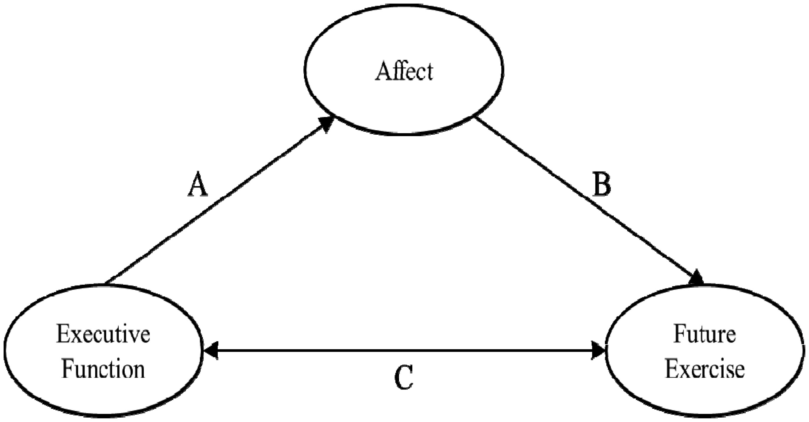
Edwards MK, Addoh O, Herod SM, et al. (2017) A Conceptual Neurocognitive Affect-Related Model for the Promotion of Exercise Among Obese Adults. Curr Obes Rep 6: 86-92. doi: 10.1007/s13679-017-0244-0
|
| [46] |
Russell JA (2003) Core affect and the psychological construction of emotion. Psychol Rev 110: 145-172. doi: 10.1037/0033-295X.110.1.145
|
| [47] |
Loprinzi PD, Herod SM, Cardinal BJ, et al. (2013) Physical activity and the brain: a review of this dynamic, bi-directional relationship. Brain Res 1539: 95-104. doi: 10.1016/j.brainres.2013.10.004
|
| [48] |
Takeuchi H, Taki Y, Sassa Y, et al. (2010) Regional gray matter volume of dopaminergic system associate with creativity: evidence from voxel-based morphometry. Neuroimage 51: 578-585. doi: 10.1016/j.neuroimage.2010.02.078
|
| [49] |
Hagger M, Chatzisarantis N, Biddle S (2002) A meta-analytic review of the theories of reasoned action and planned behavior in physical activity: Predictive validity and the contribution of additional variables. J Sport Exercise Psy 24: 3-32. doi: 10.1123/jsep.24.1.3
|
| [50] |
Gardner LA, Magee CA, Vella SA (2016) Social climate profiles in adolescent sports: Associations with enjoyment and intention to continue. J Adolesc 52: 112-123. doi: 10.1016/j.adolescence.2016.08.003
|
| [51] |
Ajzen I (1991) The theory of planned behavior. Organ Beha Hum Dec 50: 179-211. doi: 10.1016/0749-5978(91)90020-T
|
| [52] |
Smith RA, Biddle SJ (1999) Attitudes and exercise adherence: Test of the theories of reasoned action and planned behaviour. J Sports Sci 17: 269-281. doi: 10.1080/026404199365993
|
| [53] | Monteiro D, Pelletier LG, Moutão J, et al. (2018) Examining the motivational determinants of enjoyment and the intention to continue of persistent competitive swimmers. Int J Sport Psychol 49: 484-504. |
| [54] |
Rodrigues F, Teixeira DS, Neiva HP, et al. (2020) The bright and dark sides of motivation as predictors of enjoyment, intention, and exercise persistence. Scand J Medicine Sci Sports 30: 787-800. doi: 10.1111/sms.13617
|
| [55] |
Hall PA, Fong GT, Epp LJ, et al. (2008) Executive function moderates the intention-behavior link for physical activity and dietary behavior. Psychol Health 23: 309-326. doi: 10.1080/14768320701212099
|
| [56] | Hair JF, Black WC, Babin BJ, et al. (2005) Multivariate analysis of data Saddle River, NJ: Prentice-Hall. |
| [57] |
Kaufman JC (2012) Counting the muses: development of the Kaufman domains of creativity scale (K-DOCS). Psychol Aesthet Crea 6: 298. doi: 10.1037/a0029751
|
| [58] | Tan CS, Tan SA, Cheng SM, et al. (2019) Development and preliminary validation of the 20-item Kaufman domains of Creativity Scale for use with Malaysian populations. Curr Psychol 1-12. |
| [59] |
Morera OF, Stokes SM (2016) Coefficient α as a measure of test score reliability: Review of 3 popular misconceptions. Am J Public Health 106: 458-461. doi: 10.2105/AJPH.2015.302993
|
| [60] |
Kendzierski D, DeCarlo KJ (1991) Physical activity enjoyment scale: Two validation studies. J Sport Exercise Psy 13: 50-64. doi: 10.1123/jsep.13.1.50
|
| [61] |
Graves LE, Ridgers ND, Williams K, et al. (2010) The physiological cost and enjoyment of Wii Fit in adolescents, young adults, and older adults. J Phys Act Health 7: 393-401. doi: 10.1123/jpah.7.3.393
|
| [62] |
McAuley E, Courneya KS (1993) Adherence to exercise and physical activity as health-promoting behaviors: Attitudinal and self-efficacy influences. Appl Prev Psychol 2: 65-77. doi: 10.1016/S0962-1849(05)80113-1
|
| [63] |
Kang S, Lee K, Kwon S (2020) Basic psychological needs, exercise intention and sport commitment as predictors of recreational sport participants' exercise adherence. Psychol Health 35: 916-932. doi: 10.1080/08870446.2019.1699089
|
| [64] | Ball TJ, Joy EA, Gren LH, et al. (2016) Peer reviewed: concurrent validity of a self-reported physical activity “Vital Sign” questionnaire with adult primary care patients. Prev Chronic Dis 13: E16. |
| [65] | Ahmad S, Zulkurnain NNA, Khairushalimi FI (2016) Assessing the validity and reliability of a measurement model in Structural Equation Modeling (SEM). J Adv Math Comput Sci 15: 1-8. |
| [66] |
Fornell C, Larcker DF (1981) Structural equation models with unobservable variables and measurement error: Algebra and statistics. J Mark Res 18: 382-388. doi: 10.1177/002224378101800313
|
| [67] |
Schreiber JB, Nora A, Stage FK, et al. (2006) Reporting structural equation modeling and confirmatory factor analysis results: A review. J Educ Res 99: 323-338. doi: 10.3200/JOER.99.6.323-338
|
| [68] | Yuan KH, Bentler PM (2007) Robust procedures in structural equation modeling. Handbook of latent variable and related models Amsterdam: North-Holland, 367-397. |
| [69] | Gatignon H (2010) Confirmatory factor analysis, In Statistical analysis of management data New York: Springer, 59-122. |
| [70] |
Tucker LR, Lewis C (1973) A reliability coefficient for maximum likelihood factor analysis. Psychometrika 38: 1-10. doi: 10.1007/BF02291170
|
| [71] | Hayes AF (2013) Introduction to mediation, moderation, and conditional process analysis: a regression-based approach New York: Guilford Press. |
| [72] |
Preacher KJ, Hayes AF (2004) SPSS and SAS procedures for estimating indirect effects in simple mediation models. Behav Res Methods Instrum Comput 36: 717-731. doi: 10.3758/BF03206553
|
| [73] | Kline RB (2005) Structural equation modeling New York: Guilford Press. |
| [74] |
Dietrich A (2004) The cognitive neuroscience of creativity. Psychon Bull Rev 11: 1011-1026. doi: 10.3758/BF03196731
|
| [75] |
Oppezzo M, Schwartz DL (2014) Give your ideas some legs: The positive effect of walking on creative thinking. J Exp Psychol Learn Mem Cogn 40: 1142-1152. doi: 10.1037/a0036577
|
| [76] |
Kim J (2015) Physical activity benefits creativity: squeezing a ball for enhancing creativity. Creativity Res J 27: 328-333. doi: 10.1080/10400419.2015.1087258
|
| [77] | Frith E, Miller SE, Loprinzi PD (2020) Effects of Verbal Priming With Acute Exercise on Convergent Creativity. Psychol Rep 1-23. |
| [78] | Hallihan GM, Shu LHCreativity and long-term potentiation: Implications for design. (2011) .491-502. |
| [79] |
Salamone JD, Correa M (2012) The mysterious motivational functions of mesolimbic dopamine. Neuron 76: 470-485. doi: 10.1016/j.neuron.2012.10.021
|
| [80] |
Beaty RE, Benedek M, Kaufman SB, et al. (2015) Default and executive network coupling supports creative idea production. Sci Rep 5: 1-14. doi: 10.1038/srep10964
|
| [81] |
De Dreu CK, Baas M, Nijstad BA (2008) Hedonic tone and activation level in the mood-creativity link: toward a dual pathway to creativity model. J Pers Soc Psycho 94: 739-756. doi: 10.1037/0022-3514.94.5.739
|
| [82] |
Yerkes RM, Dodson JD (1908) The relation of strength of stimulus to rapidity of habit-formation. J Comp Neurol Sychol 18: 459-482. doi: 10.1002/cne.920180503
|
| [83] |
McMorris T (2016) Developing the catecholamines hypothesis for the acute exercise-cognition interaction in humans: Lessons from animal studies. Physiol Behav 165: 291-299. doi: 10.1016/j.physbeh.2016.08.011
|
| [84] |
Rhodes RE, Kates A (2015) Can the affective response to exercise predict future motives and physical activity behavior? A systematic review of published evidence. Ann Behav Med 49: 715-731. doi: 10.1007/s12160-015-9704-5
|
| [85] |
Loprinzi PD, Pazirei S, Robinson G, et al. (2020) Evaluation of a cognitive affective model of physical activity behavior. Health Promot Perspect 10: 88-93. doi: 10.15171/hpp.2020.14
|
| [86] | Fuster JM (2015) The prefrontal cortex Academic Press. |
| [87] |
Fuster JM (2002) Frontal lobe and cognitive development. J Neurocytol 31: 373-385. doi: 10.1023/A:1024190429920
|
| [88] |
Chandler DJ, Waterhouse BD, Gao WJ (2014) New perspectives on catecholaminergic regulation of executive circuits: evidence for independent modulation of prefrontal functions by midbrain dopaminergic and noradrenergic neurons. Front Neural Circuits 8: 53. doi: 10.3389/fncir.2014.00053
|
| [89] |
Pezze MA, Feldon J (2004) Mesolimbic dopaminergic pathways in fear conditioning. Prog Neurobiol 74: 301-320. doi: 10.1016/j.pneurobio.2004.09.004
|
| [90] |
Phillips AG, Ahn S, Floresco SB (2004) Magnitude of dopamine release in medial prefrontal cortex predicts accuracy of memory on a delayed response task. J Neurosci 24: 547-553. doi: 10.1523/JNEUROSCI.4653-03.2004
|
| [91] |
Goekint M, Bos I, Heyman E, et al. (2012) Acute running stimulates hippocampal dopaminergic neurotransmission in rats, but has no influence on brain-derived neurotrophic factor. J Appl Physiol 112: 535-541. doi: 10.1152/japplphysiol.00306.2011
|
| [92] |
Chang YK, Labban JD, Gapin JI, et al. (2012) The effects of acute exercise on cognitive performance: a meta-analysis. Brain Res 1453: 87-101. doi: 10.1016/j.brainres.2012.02.068
|
| [93] |
Stevens DJ, Arciuli J, Anderson DI (2015) Concurrent movement impairs incidental but not intentional statistical learning. Cogn Sci 39: 1081-1098. doi: 10.1111/cogs.12180
|
| [94] |
Daikoku T, Takahashi Y, Futagami H, et al. (2017) Physical fitness modulates incidental but not intentional statistical learning of simultaneous auditory sequences during concurrent physical exercise. Neurol Res 39: 107-116. doi: 10.1080/01616412.2016.1273571
|
| [95] | Mayesky M (2011) Creative activities for young children Cengage Learning. |
Figures(3) / Tables(5)

Myungjin Jung, Han Soo Kim, Paul D Loprinzi, Minsoo Kang. Serial-multiple mediation of enjoyment and intention on the relationship between creativity and physical activity[J]. AIMS Neuroscience, 2021, 8(1): 161-180. doi: 10.3934/Neuroscience.2021008


 DownLoad: