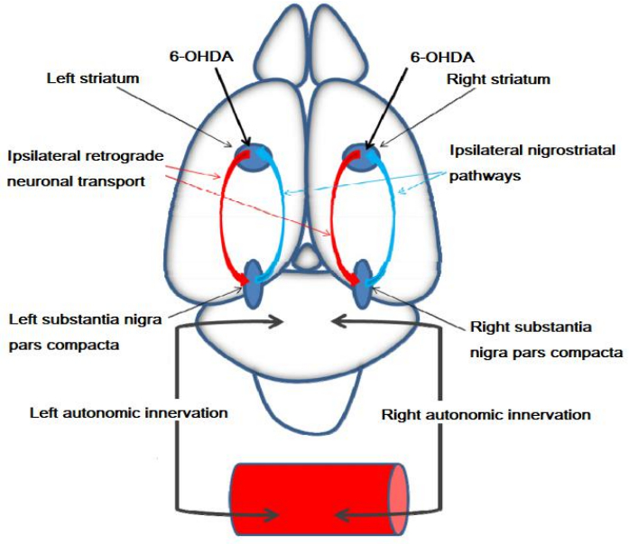
Parkinson’s disease, one of the most common neurodegenerative diseases, characterized by unilateral brain dopamine damage in its initial stages, remains unknown in many respects. It is especially necessary to improve the early diagnosis and, in order to improve the treatment, to go thoroughly into the knowledge of its pathophysiology. To do this, it is essential to perform studies in appropriate animal models of the disease. One of those is generated by the unilateral intracerebral administration of the neurotoxic 6-hydroxydopamine that produces clear asymmetrical cerebral dopamine depletion. Currently the neuronal coexistence of several neurotransmitters is obvious. Particularly interesting is the coexistence of dopamine with various neuropeptides. If the neuronal content of dopamine is asymmetrically altered in the early stages of the Parkinson’s disease, the coexisting neuropeptides may also be asymmetrically altered. Therefore, their study is important to appropriately understand the pathogenesis of the Parkinson’s disease. The function of the neuropeptides can be studied through their metabolism by neuropeptidases whose activity reflects the functional status of their endogenous substrates as well as the one of the peptides resulting from their hydrolysis. Here we review the 6-hydroxydopamine model of experimental hemiparkinsonism as an appropriate model to study the initial asymmetric stages of the disease. In particular, we analyze the consequences of unilateral brain dopamine depletions on the functionality of brain neuropeptides through the study of the activity of cerebral neuropeptidases.
Citation: I. Banegas, I. Prieto, A.B. Segarra, M. de Gasparo, M. Ramírez-Sánchez. Study of the Neuropeptide Function in Parkinson’s Disease Using the 6-Hydroxydopamine Model of Experimental Hemiparkinsonism[J]. AIMS Neuroscience, 2017, 4(4): 223-237. doi: 10.3934/Neuroscience.2017.4.223
Parkinson’s disease, one of the most common neurodegenerative diseases, characterized by unilateral brain dopamine damage in its initial stages, remains unknown in many respects. It is especially necessary to improve the early diagnosis and, in order to improve the treatment, to go thoroughly into the knowledge of its pathophysiology. To do this, it is essential to perform studies in appropriate animal models of the disease. One of those is generated by the unilateral intracerebral administration of the neurotoxic 6-hydroxydopamine that produces clear asymmetrical cerebral dopamine depletion. Currently the neuronal coexistence of several neurotransmitters is obvious. Particularly interesting is the coexistence of dopamine with various neuropeptides. If the neuronal content of dopamine is asymmetrically altered in the early stages of the Parkinson’s disease, the coexisting neuropeptides may also be asymmetrically altered. Therefore, their study is important to appropriately understand the pathogenesis of the Parkinson’s disease. The function of the neuropeptides can be studied through their metabolism by neuropeptidases whose activity reflects the functional status of their endogenous substrates as well as the one of the peptides resulting from their hydrolysis. Here we review the 6-hydroxydopamine model of experimental hemiparkinsonism as an appropriate model to study the initial asymmetric stages of the disease. In particular, we analyze the consequences of unilateral brain dopamine depletions on the functionality of brain neuropeptides through the study of the activity of cerebral neuropeptidases.

| [1] | Segarra AB, Banegas I, Prieto I, et al. (2016) [Brain asymmetry and dopamine: beyond motor implications in Parkinson's disease and experimental hemiparkinsonism]. Rev Neurol 63: 415-421. |
| [2] |
Bové J, Prou D, Perier C, et al. (2005) Toxin-Induced Models of Parkinson's Disease. NeuroRx 2: 484-494. doi: 10.1602/neurorx.2.3.484

|
| [3] | Zhang J, Goodlett DR, Montine TJ (2005) Proteomic biomarker discovery in cerebrospinal fluid for neurodegenerative diseases. J Alzheimers Dis 8: 377-386. |
| [4] |
Goldstein A, Lowney LI, Pal BK (1971) Stereospecific and nonspecific interactions of the morphine congener levorphanol in subcellular fractions of mouse brain. Proc Natl Acad Sci U S A 68: 1742-1747. doi: 10.1073/pnas.68.8.1742
|
| [5] |
Pert CB, Snyder SH (1973) Properties of opiate-receptor binding in rat brain. Proc Natl Acad Sci U S A 70: 2243-2247. doi: 10.1073/pnas.70.8.2243
|
| [6] | Simon EJ, Hiller JM, Edelman I (1973) Stereospecific binding of the potent narcotic analgesic (3H) Etorphine to rat-brain homogenate. Proc Natl Acad Sci U S A 70: 1947-1949. |
| [7] | Hughes J, Smith TW, Kosterlitz HW, et al. (1975) Identification of two related pentapeptides from the brain with potent opiate agonist activity. Nature 258: 577-580. |
| [8] | Merighi A (2002) Costorage and coexistence of neuropeptides in the mammalian CNS. Prog Neurobiol 66: 161-190. |
| [9] |
Burbach JP (2011) What are neuropeptides? Methods Mol Biol 789: 1-36. doi: 10.1007/978-1-61779-310-3_1
|
| [10] | Cuello AC (1982) Co-transmission McMillan, London. |
| [11] | Chan-Palay V, Palay SL (1984) Coexistence of Neuroactive Substances in Neurons Wiley, New York. |
| [12] |
Hökfelt T, Millhorn D, Seroogi K, et al. (1987) Coexistence of peptides with classical neurotransmitters. Experientia 43: 768-780. doi: 10.1007/BF01945354
|
| [13] | Dale HH (1935) Pharmacology and nerve-endings. Walter Ernest Dixon Memorial Lecture for 1934. Proc R Soc Med Therap Sect 28: 319-332. |
| [14] |
Everitt BJ, Meister B, Hökfelt T, et al. (1986) The hypothalamic arcuate nucleus- median eminence complex: immunohistochemistry of transmitters, peptides and DARPP-32 with special reference to coexistence in dopamine neurons. Brain Res 396: 97-155. doi: 10.1016/0165-0173(86)90001-9
|
| [15] |
Hökfelt T, Everitt BJ, Theodorsson-Norheim E, et al. (1984) Occurrence of neurotensinlike immunoreactivity in subpopulations of hypothalamic, mesencephalic, and medullary catecholamine neurons. J Comp Neurol 222: 543-559. doi: 10.1002/cne.902220407
|
| [16] | Hökfelt T, Skirboll L, Rehfeld JF, et al. (1980) A subpopulation of mesencephalic dopamine neurons projecting to limbic areas contains a cholecystokinin-like peptide: evidence from immunohistochemistry combined with retrograde tracing. Neuroscience 5: 2093-2124. |
| [17] |
Seroogy KB, Ceccatelli S, Schalling M (1988) A subpopulation of dopaminergic neurons in rat ventral mesencephalon contains both neurotensin and cholecystokinin. Brain Res 455: 88-98. doi: 10.1016/0006-8993(88)90117-5
|
| [18] | Salio C, Lossi L, Ferrini F, et al. (2006) Neuropeptides as synaptic transmitters. Cell Tissue Res 326: 583-598. |
| [19] | Jonsson G (1983) Chemical lesioning techniques: monoamine neurotoxins. In: Handbook of chemical neuroanatomy. Methods in chemical neuroanatomy (Björklund A, Hökfelt T, eds), Amsterdam: Elsevier Science Publishers BV: 463-507. |
| [20] | Cohen G (1984) Oxy-radical toxicity in catecholamine neurons. Neurotoxicology 5: 77-82. |
| [21] | Przedborski S, Ischiropoulos H (2005) Reactive oxygen and nitrogen species: weapons of neuronal destruction in models of Parkinson's disease. Antioxid Redox Signal 7: 685-693. |
| [22] | Ungerstedt U (1971) Adipsia and aphagia after 6-hydroxydopamine induced degeneration of the nigro-striatal dopamine system. Acta Physiol Scand Suppl 367: 95-122. |
| [23] | Ungerstedt U (1968) 6-Hydroxydopamine induced degeneration of central monoamine neurons. Eur J Pharmacol 5: 107-110. |
| [24] | Javoy F, Sotelo C, Herbert A, et al. (1976) Specificity of dopaminergic neuronal degeneration induced by intracerebral injection of 6-hydroxydopamine in the nigrostriatal dopamine system. Brain Res 102: 210-215. |
| [25] |
Jeon BS, Jackson-Lewis V, Burke RE (1995) 6-Hydroxydopamine lesion of the rat substantia nigra: time course and morphology of cell death. Neurodegeneration 4: 131-137. doi: 10.1006/neur.1995.0016
|
| [26] | Sarre S, Yuan H, Jonkers N, et al. (2004) in vivo characterization of somatodendritic dopamine release in the substantia nigra of 6-hydroxydopamine- lesioned rats. J Neurochem 90: 29-39. |
| [27] |
Przedborski S, Levivier M, Jiang H, et al. (1995) Dose-dependent lesions of the dopaminergic nigrostriatal pathway induced by intrastriatal injection of 6-hydroxydopamine. Neuroscience 67: 631-647. doi: 10.1016/0306-4522(95)00066-R
|
| [28] |
Stromberg I, Bjorklund H, Dahl D, et al. (1986) Astrocyte responses to dopaminergic denervations by 6-hydroxydopamine and 1-methyl-4-phenyl-1,2,3,6-tetrahydropyridine as evidenced by glial fibrillary acidic protein immunohistochemistry. Brain Res Bull 17: 225-236. doi: 10.1016/0361-9230(86)90119-X
|
| [29] |
Rodriguez DM, Abdala P, Barroso-Chinea P, et al. (2001) Motor behavioural changes after intracerebroventricular injection of 6-hydroxydopamine in the rat: an animal model of Parkinson's disease. Behav Brain Res 122: 79-92. doi: 10.1016/S0166-4328(01)00168-1
|
| [30] |
Ungerstedt U, Arbuthnott G (1970) Quantitative recording of rotational behaviour in rats after 6-hydroxydopamine lesions of the nigrostriatal dopamine system. Brain Res 24: 485-493. doi: 10.1016/0006-8993(70)90187-3
|
| [31] | Jiang H, Jackson-Lewis V, Muthane U, et al. (1993) Adenosine receptor antagonists potentiate dopamine receptor agonist-induced rotational behavior in 6-hydroxydopamine-lesioned rats. Brain Res 613: 347-351. |
| [32] |
Papa SM, Engber TM, Kask AM, et al. (1994) Motor fluctuations in levodopa treated parkinsonian rats: relation to lesion extent and treatment duration. Brain Res 662: 69-74. doi: 10.1016/0006-8993(94)90796-X
|
| [33] | Jolicoeur FB, Rivest R (1992) Rodent model of Parkinson's disease. In: Boulto AA, Bakerand a GB, Butterworth RF (Eds.). Neuromethods 21, Animal Models of Neurological Disease I, Totowa, NJ: Humana Press: 135-158. |
| [34] | Paxinos G, Watson C (1998) The rat brain in stereotaxic coordinates. 4th Ed. London: Academic Press. |
| [35] |
Deumens R, Blokland A, Prickaerts J (2002) Modeling Parkinson's disease in rats: an evaluation of 6-OHDA lesions of the nigrostriatal pathway. Exp Neurol 175: 303-317. doi: 10.1006/exnr.2002.7891
|
| [36] | Berger K, Przedborski S, Cadet JL (1991) Retrograde degeneration of nigrostriatal neurons induced by intraestriatal 6-hydroxydopamine injection in rats. Brain Res Bull 25: 301-307. |
| [37] | Luthman J, Brodin E, Sundström E, et al. (1990) Studies on brain monoamine and neuropeptide systems after neonatal intracerebroventricular 6-hydroxydopamine treatment. Int J Dev Neurosci 8: 549-560. |
| [38] | Martorana A, Fusco FR, D'Angelo V, et al. (2003) Enkephalin, neurotensin, and substance P immunoreactivite neurones of the rat GP following 6-hydroxydopamine lesion of the substantia nigra. Exp Neurol 183: 311-319. |
| [39] | Petkova-Kirova P, Giovannini MG, Kalfin R, et al. (2012) Modulation of acetylcholine release by cholecystokinin in striatum: receptor specificity; role of dopaminergic neuronal activity. Brain Res Bull 89: 177-184. |
| [40] |
You ZB, Herrera-Marschitz M, Pettersson E, et al. (1996) Modulation of neurotransmitter release by cholecystokinin in the neostriatum and substantia nigra of the rat: regional and receptor specificity. Neuroscience 74: 793-804. doi: 10.1016/0306-4522(96)00149-2
|
| [41] |
Kimura Y, Miyake K, Kitaura T, et al. (1994) Changes of cholecystokinin octapeptide tissue levels in rat brain following dopamine neuron lesions induced by 6-hydroxydopamine. Biol Pharm Bull 17: 1210-1214. doi: 10.1248/bpb.17.1210
|
| [42] | Artaud F, Baruch P, Stutzmann JM, et al. (1989) Cholecystokinin: Corelease with dopamine from nigrostriatal neurons in the cat. Eur J Neurosci 1: 162-171. |
| [43] | Merighi A (2011) Neuropeptides. Methods and Protocols. Springer Protocols. New York: Humana Press. |
| [44] |
Ramírez M, Prieto I, Banegas I, et al. (2011) Neuropeptidases. Methods Mol Biol 789: 287-294. doi: 10.1007/978-1-61779-310-3_18
|
| [45] | Checler F (1993) Methods in neurotransmitter and neuropeptide research, Parvez SH, Naoi M, Nagatsu T, Parvez S eds. Amsterdam: Elsevier. |
| [46] | White JD, Stewart KD, Krause JE, et al. (1985) Biochemistry of peptide-secreting neurons. Physiol Rev 65: 553-606. |
| [47] |
Horsthemke B, Hamprecht B, Bauer K (1983) Heterogeneous distribution of enkephalin-degrading peptidases between neuronal and glial cells. Biochem Biophys Res Commun 115: 423-429. doi: 10.1016/S0006-291X(83)80161-2
|
| [48] | Arechaga G, Sánchez B, Alba F, et al. (1995) Subcellular distribution of soluble and membrane-bound Arg-beta-naphthylamide hydrolyzing activities in the developing and aged rat brain. Cell Mol Biol Res 41: 369-375. |
| [49] |
Hallberg M (2015) Neuropeptides: metabolism to bioactive fragments and the pharmacology of their receptors. Med Res Rev 35: 464-519. doi: 10.1002/med.21323
|
| [50] |
Prieto I, Villarejo AB, Segarra AB, et al. (2015) Tissue distribution of CysAP activity and its relationship to blood pressure and water balance. Life Sci 134: 73- 78. doi: 10.1016/j.lfs.2015.04.023
|
| [51] | Marinus J, Van Hilten JJ (2015) The significance of motor asymmetry in Parkinson's disease. Mov Disord 30: 379-385. |
| [52] |
Okada M, Kato T (1985) Peptidase-containing neurons in rat striatum. Neurosci Res 2: 421-433. doi: 10.1016/0168-0102(85)90015-X
|
| [53] |
Banegas I, Prieto I, Vives F et al. (2010) Lateralized response of oxytocinase activity in the medial prefrontal cortex of a unilateral rat model of Parkinson's disease. Behav Brain Res 213: 328-231. doi: 10.1016/j.bbr.2010.05.030
|
| [54] | Durand M, Berton O, Aguerre S, et al. (1999) Effects of repeated fluoxetine on anxiety-related behaviours, central serotonergic systems, and the corticotropic axis in SHR and WKY rats. Neuropharmacology 38: 893-907. |
| [55] |
Banegas I, Prieto I, Segarra AB, et al. (2017) Bilateral distribution of enkephalinase activity in the medial prefrontal cortex differs between WKY and SHR rats unilaterally lesioned with 6-hydroxydopamine. Prog Neuropsychopharmacol Biol Psychiatry 75: 213-218. doi: 10.1016/j.pnpbp.2017.02.015
|
| [56] | Gerendai I, Halász B (2001) Asymmetry of the neuroendocrine system. News Physiol Sci 16: 92-95. |
| [57] | Banegas I, Prieto I, Vives F, et al. (2004) Plasma aminopeptidase activities in rats after left and right intrastriatal administration of 6-hydroxydopamine. Neuroendocrinology 80: 219-224. |
| [58] | Toda N, Okamura T (2003). The pharmacology of nitric oxide in the peripheral nervous system of blood vessels. Pharmacol Rev 55: 271-324. |
| [59] | Raij L (2001) Hypertension and cardiovascular risk factors: role of the angiotensin II-nitric oxide interaction. Hypertension 37: 767-773. |
| [60] | Jenkins TA, Allen AM, Chai SY, et al. (1996) Interactions of angiotensin II with central dopamine. Adv Exp Med Biol 396: 93-103. |
| [61] |
Berg T (2005) Increased counteracting effect of eNOS and nNOS on an alpha1- adrenergic rise in total peripheral vascular resistance in spontaneous hypertensive rats. Cardiovasc Res 67: 736-744. doi: 10.1016/j.cardiores.2005.04.006
|
| [62] | Banegas I, Prieto I, Vives F et al. (2009) Asymmetrical response of aminopeptidase A and nitric oxide in plasma of normotensive and hypertensive rats with experimental hemiparkinsonism. Neuropharmacology 56: 573-579. |
| [63] | Banegas I, Prieto I, Segarra AB, et al. (2011) Blood pressure increased dramatically in hypertensive rats after left hemisphere lesions with 6-hydroxydopamine. Neurosci Lett 500: 148-150. |
| [64] | Banegas I, Barrero F, Durán R, et al. (2006) Plasma aminopeptidase activities in Parkinson's disease. Horm Metab Res 38: 758-760. |
| [65] |
Duran R, Barrero FJ, Morales B, et al. (2011) Oxidative stress and aminopeptidases in Parkinson's disease patients with and without treatment. Neurodegener Dis 8: 109-116. doi: 10.1159/000315404
|
Figures(2)

I. Banegas, I. Prieto, A.B. Segarra, M. de Gasparo, M. Ramírez-Sánchez. Study of the Neuropeptide Function in Parkinson’s Disease Using the 6-Hydroxydopamine Model of Experimental Hemiparkinsonism[J]. AIMS Neuroscience, 2017, 4(4): 223-237. doi: 10.3934/Neuroscience.2017.4.223


 DownLoad: