Housing price dynamics and elasticities: Portugal's conundrum

António M. Cunha; Ricardo Loureiro; António M. Cunha; Ricardo Loureiro

doi:10.3934/NAR.2024004

National Accounting Review

2024, Volume 6, Issue 1: 75-94. doi: 10.3934/NAR.2024004

Previous Article Next Article

Research article

Housing price dynamics and elasticities: Portugal's conundrum

António M. Cunha ^{1
,
,},
Ricardo Loureiro ²

1.
ISAG – European Business School and CICET – Research Center in Business Sciences and Tourism, Centre for Organizational and Social Studies of Polytechnic of Porto (CEOS.PP), Porto, Portugal
2.
ISCAP – Porto Accounting and Business School, Polytechnic University of Porto, Porto, Portugal

Received: 20 December 2023 Revised: 21 January 2024 Accepted: 31 January 2024 Published: 06 February 2024
JEL Codes: E10, R31

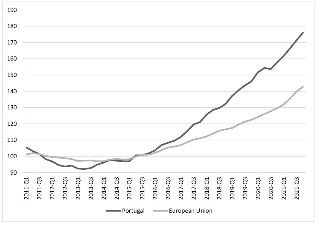
We aimed to estimate the housing price determinants and elasticities in Portugal's metropolitan areas to help understand the dynamics of the abnormal price increase of the last decade, one of the highest in Europe and the World.

We followed a three-step methodology applying panel data and time series regression estimation. First, we estimated the determinants of housing prices at the national and metropolitan area levels. Second, we split the sample by coastal and inner metropolitan areas and estimated the determinants of housing prices and the supply elasticities of each group. Third, we estimated the correlations between housing price growth and elasticities to find whether these determinants correlate.

The results showed that at the national level, housing prices are inelastic to aggregate income (0.112). Momentum is the most significant determinant of housing prices (0.760). At the metropolitan areas level, we found an inelastic housing supply, a price-to-income elasticity close to zero, and a more inelastic supply in coastal areas. We found no significant correlation between housing price growth, price-to-income, and supply elasticity. The coastal areas registered housing price growth and a momentum effect much higher than the inner areas, suggesting the existence of dynamic speculative forces that cause prices to move beyond what can be explained by equilibrium models.

The present study contributes to the literature on housing price dynamics by showing that the conventional equilibrium stock-flow model does not explain the increase in Portugal's current housing prices, suggesting that other forces (such as economic uncertainty and sentiment) determine the housing price dynamics. The explanation for the housing price growth in Portugal is a conundrum. We believe this knowledge can help define better housing policies at the local and national levels.
- housing price dynamics,
- elasticities,
- housing market determinants
Citation: António M. Cunha, Ricardo Loureiro. Housing price dynamics and elasticities: Portugal's conundrum[J]. National Accounting Review, 2024, 6(1): 75-94. doi: 10.3934/NAR.2024004

Related Papers:

Abstract

We aimed to estimate the housing price determinants and elasticities in Portugal's metropolitan areas to help understand the dynamics of the abnormal price increase of the last decade, one of the highest in Europe and the World.

We followed a three-step methodology applying panel data and time series regression estimation. First, we estimated the determinants of housing prices at the national and metropolitan area levels. Second, we split the sample by coastal and inner metropolitan areas and estimated the determinants of housing prices and the supply elasticities of each group. Third, we estimated the correlations between housing price growth and elasticities to find whether these determinants correlate.

The results showed that at the national level, housing prices are inelastic to aggregate income (0.112). Momentum is the most significant determinant of housing prices (0.760). At the metropolitan areas level, we found an inelastic housing supply, a price-to-income elasticity close to zero, and a more inelastic supply in coastal areas. We found no significant correlation between housing price growth, price-to-income, and supply elasticity. The coastal areas registered housing price growth and a momentum effect much higher than the inner areas, suggesting the existence of dynamic speculative forces that cause prices to move beyond what can be explained by equilibrium models.

The present study contributes to the literature on housing price dynamics by showing that the conventional equilibrium stock-flow model does not explain the increase in Portugal's current housing prices, suggesting that other forces (such as economic uncertainty and sentiment) determine the housing price dynamics. The explanation for the housing price growth in Portugal is a conundrum. We believe this knowledge can help define better housing policies at the local and national levels.

References

[1]	Aastveit KA, Albuquerque B, Anundsen AK (2023) Changing Supply Elasticities and Regional Housing Booms. J Money Credit Banking 55: 1749–1783. https://doi.org/10.1111/jmcb.13009 doi: 10.1111/jmcb.13009
[2]	Adams Z, Füss R (2010) Macroeconomic Determinants of International Housing Markets. J Hous Econ 19: 38–50. https://doi.org/10.1016/j.jhe.2009.10.005 doi: 10.1016/j.jhe.2009.10.005
[3]	Balcilar M, Bouri E, Gupta R, et al. (2021a) High-Frequency Predictability of Housing Market Movements of the United States: The Role of Economic Sentiment. J Behav Financ 22: 490–498. https://doi.org/10.1080/15427560.2020.1822359 doi: 10.1080/15427560.2020.1822359
[4]	Balcilar M, Roubaud D, Uzuner G, et al. (2021b) Housing sector and economic policy uncertainty: a GMM panel VAR approach. Int Rev Econ Finance 76: 114–126. https://doi.org/10.1016/j.iref.2021.05.011 doi: 10.1016/j.iref.2021.05.011
[5]	Belke A, Keil J (2018) Fundamental Determinants of Real Estate Prices: A Panel Study of German Regions. Int Adv Econ Res 24: 25–45. https://doi.org/10.1007/s11294-018-9671-2 doi: 10.1007/s11294-018-9671-2
[6]	Beracha E, Skiba H (2011) Momentum in Residential Real Estate. J Real Estate Finance Econ 43: 299–320. https://doi.org/10.1007/s11146-009-9210-2 doi: 10.1007/s11146-009-9210-2
[7]	Bramley G (1993) Land use planning and the housing market in Britain – the impact on house building and house prices. Environ Plann A 25: 1021–1052. https://doi.org/10.1068/a251021 doi: 10.1068/a251021
[8]	Caldera A, Johansson Å (2013) The price responsiveness of housing supply in OECD countries. J Hous Econ 22: 231–249. https://doi.org/10.1016/j.jhe.2013.05.002 doi: 10.1016/j.jhe.2013.05.002
[9]	Case B, Wachter S (2005) Residential real estate price indices as financial soundness indicators: methodological issues. BIS papers 21: 197–211.
[10]	Case KE, Shiller RJ (1989) The Efficiency of the Market for Single-Family Homes. Am Econ Rev 79: 125–137. https://doi.org/10.3386/w2506 doi: 10.3386/w2506
[11]	Case KE, Shiller RJ (1990) Forecasting Prices and Excess Returns in the Housing Market. Real Estate Econ 18: 253–273. https://doi.org/10.1111/1540-6229.00521 doi: 10.1111/1540-6229.00521
[12]	Case KE, Shiller RJ (2003) Is there a bubble in the housing market? Brookings Pap Econ Act 2: 299–362. https://doi.org/10.1353/eca.2004.0004 doi: 10.1353/eca.2004.0004
[13]	Chowdhury SR, Gupta K, Tzeremes P (2023) US housing prices and the transmission mechanism of connectedness. Finance Res Lett 58: 104636. https://doi.org/10.1016/j.frl.2023.104636 doi: 10.1016/j.frl.2023.104636
[14]	Cohen V, Karpaviciute L (2016) The analysis of the determinants of housing prices. Indep J Manag Prod 8: 49–63. https://doi.org/10.14807/ijmp.v8i1.521 doi: 10.14807/ijmp.v8i1.521
[15]	Cunha AM, Lobã o J (2021a) The determinants of real estate prices in The European context: A four-level analysis. J Eur Real Estate Res 14: 331–348. https://doi.org/10.1108/JERER-10-2020-0053 doi: 10.1108/JERER-10-2020-0053
[16]	Cunha AM, Lobã o J (2021b) The effects of tourism on housing prices: applying a difference-in-differences methodology to the Portuguese market. Int J Hous Mark Anal 15: 762–779. https://doi.org/10.1108/IJHMA-04-2021-0047 doi: 10.1108/IJHMA-04-2021-0047
[17]	Cunha AM, Lobã o J (2022) House price dynamics in Iberian Metropolitan Statistical Areas: slope heterogeneity, cross-sectional dependence and elasticities. J Eur Real Estate Res 15: 444–462. https://doi.org/10.1108/JERER-02-2022-0005 doi: 10.1108/JERER-02-2022-0005
[18]	Deng KK, Wong SK (2021) Revisiting the Autocorrelation of Real Estate Returns. J Real Estate Finan Econ 67: 243–263. https://doi.org/10.1007/s11146-021-09830-8 doi: 10.1007/s11146-021-09830-8
[19]	DiPasquale D, Wheaton WC (1992) The markets for real estate assets and space: a conceptual framework. Real Estate Econ 20: 181–198. https://doi.org/10.1111/1540-6229.00579 doi: 10.1111/1540-6229.00579
[20]	DiPasquale D, Wheaton WC (1994) Housing market dynamics and the future of housing prices. J Urban Econ 35: 1–27. https://doi.org/10.1006/juec.1994.1001 doi: 10.1006/juec.1994.1001
[21]	Dröes MI, Francke MK (2018) What causes the positive price-turnover correlation in European housing markets? J Real Estate Finance Econ 57: 618–646. https://doi.org/10.1007/s11146-017-9602-7 doi: 10.1007/s11146-017-9602-7
[22]	Duca JV (2020) Making sense of increased synchronization in global house prices. J Eur Real Estate Res 13: 5–16, https://doi.org/10.1108/JERER-11-2019-0044 doi: 10.1108/JERER-11-2019-0044
[23]	Follain JR (1979) The Price Elasticity of the Long Run Supply of New Housing Construction. Land Econ 55: 190–199. https://doi.org/10.2307/3146061 doi: 10.2307/3146061
[24]	Gabauer D, Gupta R, Marfatia HA, et al. (2024). Estimating U.S. housing price network connectedness: Evidence from dynamic Elastic Net, Lasso, and ridge vector autoregressive models. Int Rev Econ Finance 89: 349–362. https://doi.org/10.1016/j.iref.2023.10.013 doi: 10.1016/j.iref.2023.10.013
[25]	Goodman AC (2005) The other side of eight miles: suburban population and housing supply. Real Estate Econ 33: 539–569. https://doi.org/10.1111/j.1540-6229.2005.00129.x doi: 10.1111/j.1540-6229.2005.00129.x
[26]	Gray D (2021) Medium-term cycles in affordability: what does the house price to income ratio indicate? National Accounting Review 3: 204–217. https://doi.org/10.3934/NAR.2021010 doi: 10.3934/NAR.2021010
[27]	Gray D (2023) Housing market activity diffusion in England and Wales. National Accounting Review 5: 125–144. https://doi.org/10.3934/NAR.2023008 doi: 10.3934/NAR.2023008
[28]	Green R, Malpezzi S, Mayo S (2005) Metropolitan-Specific Estimates of the Price Elasticity of Supply of Housing, and Their Sources. Am Econ Rev 95: 334–339. https://doi.org/10.1257/000282805774670077 doi: 10.1257/000282805774670077
[29]	Gupta R, Lau CKM, Nyakabawo W (2020) Predicting aggregate and state-level US house price volatility: the role of sentiment. J Rev Global Econ 9: 30–46. https://doi.org/10.6000/1929-7092.2020.09.05 doi: 10.6000/1929-7092.2020.09.05
[30]	Holly S, Pesaran MH, Yamagata T (2010) A spatio-temporal model of house prices in the USA. J Econom 158: 160–173. https://doi.org/10.1016/j.jeconom.2010.03.040 doi: 10.1016/j.jeconom.2010.03.040
[31]	Jud GD, Winkler DT (2002) The Dynamics of Metropolitan Housing Prices. J Real Estate Res 23: 29–46. https://www.jstor.org/stable/24887611
[32]	Kishor NK, Marfatia HA (2017) The dynamic relationship between housing pricesand the macroeconomy: Evidence from OECD countries. J Real Estate Finan Econ 54: 237–268. https://doi.org/10.1007/s11146-015-9546-8
[33]	Li Q, Chand S (2013) Housing prices and market fundamentals in urban China. Habitat Int 40: 148–153. https://doi.org/10.1016/j.habitatint.2013.04.002 doi: 10.1016/j.habitatint.2013.04.002
[34]	Marfatia HA (2021) Modeling House Price Synchronization across the U.S. states and their Time-Varying Macroeconomic Linkages. J Time Ser Econ 13: 73–117. https://doi.org/10.1515/jtse-2017-0014
[35]	Meen G (2005) On the Economics of the Barker Review of Housing Supply. Housing Stud 20: 949–971. https://doi.org/10.1080/02673030500291082 doi: 10.1080/02673030500291082
[36]	Muth RF (1960) The demand for non-farm housing, In: Harberger, A.C. (Ed.), The Demand for Durable Goods, Chicago: University of Chicago Press, 27–96.
[37]	Ngene GM, Gupta R (2023) Impact of housing price uncertainty on herding behavior: evidence from UK's regional housing markets. J Hous Built Environ 38: 931–949. https://doi.org/10.1007/s10901-022-09975-9 doi: 10.1007/s10901-022-09975-9
[38]	Nyakabawo W, Gupta R, Marfatia HA (2018) High frequency impact of monetary policy and macroeconomic surprises on US MSAs, aggregate US housing returns and asymmetric volatility. Advances in Decision Sciences 22: 1–25.
[39]	Oikarinen E, Bourassa SC, Hoesli M, Engblom J (2018) US Metropolitan House Price Dynamics. J Urban Econ 105: 54–69. https://doi.org/10.1016/j.jue.2018.03.001 doi: 10.1016/j.jue.2018.03.001
[40]	Oikarinen E, Engblom J (2016) Differences in housing price dynamics across cities: The comparison of different panel model specifications. Urban Stud 53: 2312–2329. https://doi.org/10.1177/0042098015589883 doi: 10.1177/0042098015589883
[41]	Paciorek A (2013) Supply constraints and housing market dynamics. J Urban Econ 77: 11–26. https://doi.org/10.1016/j.jue.2013.04.001 doi: 10.1016/j.jue.2013.04.001
[42]	Peng A, Wheaton W (1994) Effects of restrictive land supply on housing in Hong Kong: an econometric analysis. J Hous Res 5: 263–291.
[43]	Quigley JM (1999) Real estate prices and economic cycles. Int Real Estate Rev 2: 1–20.
[44]	Sherlock E (2023) As UK House Prices Continue to Rise: These are the Most Unaffordable Housing Markets Worldwide. Available from: https://moneytransfers.com/news/2023/11/07/as-uk-house-prices-continue-to-rise-these-are-the-most-unaffordable-housing-markets-worldwide.
[45]	Sims CA (1980) Macroeconomics and Reality. Econometrica 48: 1–48. https://doi.org/10.2307/1912017 doi: 10.2307/1912017
[46]	Stover M (1986) The Price Elasticity of the Supply of Single-Family Detached Urban Housing. J Urban Econ 20: 331–340. https://doi.org/10.1016/0094-1190(86)90023-9 doi: 10.1016/0094-1190(86)90023-9
[47]	Taltavull de La Paz P (2003) Determinants of housing prices in Spanish cities. J Prop Invest Financ 21: 109–135. https://doi.org/10.1108/14635780310469102 doi: 10.1108/14635780310469102
[48]	Tavares FO, Pereira ET, Moreira AC (2014) The Portuguese residential real estate market. an evaluation of the last decade. Panoeconomicus 61: 739–757. https://doi.org/10.2298/PAN1406739T
[49]	Turk A (2015) Housing price and household debt interactions in Sweden. Int Monetary Fund 2015: 1–44. https://doi.org/10.5089/9781513586205.001 doi: 10.5089/9781513586205.001
[50]	Wang S, Chan SH, Xu B (2012) The Estimation and Determinants of the Price Elasticity of Housing Supply: Evidence from China. J Real Estate Res 34: 311–344. https://doi.org/10.1080/10835547.2012.12091336 doi: 10.1080/10835547.2012.12091336
[51]	Read S (2022) House prices and rents have soared in the EU since 2010. Will rising interest rates pull them back down? Available from: https://www.weforum.org/agenda/2022/08/house-price-rent-europe/.
[52]	Tzeremes P (2021) The Asymmetric Effects of Regional House Prices in the UK: New Evidence from Panel Quantile Regression Framework. Stud Microecon 10: 7–22. https://doi.org/10.1177/2321022220980541 doi: 10.1177/2321022220980541

Reader Comments

Your name:*

Email:*
© 2024 the Author(s), licensee AIMS Press. This is an open access article distributed under the terms of the Creative Commons Attribution License (http://creativecommons.org/licenses/by/4.0)