Financing low-carbon hydrogen: The role of public policies and strategies in the EU, UK and USA

João Moura; Isabel Soares; João Moura; Isabel Soares

doi:10.3934/GF.2023011

Green Finance

2023, Volume 5, Issue 2: 265-297. doi: 10.3934/GF.2023011

Previous Article Next Article

Research article Special Issues

Financing low-carbon hydrogen: The role of public policies and strategies in the EU, UK and USA

João Moura ^{1
,
,},
Isabel Soares ²

1.
Center for Economics and Finance at University of Porto (CEF.UP), Portugal
2.
CEF.UP and School of Economics of the University of Porto (FEP), Porto, Portugal

Received: 21 April 2023 Revised: 12 June 2023 Accepted: 20 June 2023 Published: 28 June 2023
JEL Codes: Q28, Q42, Q48

The goal of this study is twofold: first, to understand the rationales of public policies and possible outcomes on energy systems design behind supporting national hydrogen strategies in three major economic blocs (the EU, UK and USA) and possible outcomes on energy systems design; second, to identify differences in policy approaches to decarbonization through H₂ promotion. Large-scale expansion of low-carbon H₂ demands careful analysis and understanding of how public policies can be fundamental drivers of change. Our methodological approach was essentially economic, using the International Energy Agency (IEA) policy database as a main information source. First, we identified all regional policies and measures that include actions related to H₂, either directly or indirectly. Then, we reclassified policy types, sectors and technologies to conduct a comparative analysis which allowed us to reduce the high degree of economic ambiguity in the database. Finally, we composed a detailed discussion of our findings. While the EU pushed for renewable H₂, the UK immediately targeted low-carbon H₂ solutions, equally considering both blue and green alternatives. The USA pursues a clean H₂ economy based on both nuclear and CCS fossil technology. Although there is a general focus on fiscal and financing policy actions, distinct intensities were identified, and the EU presents a much stricter regulatory framework than the UK and USA. Another major difference between blocs concerns target sectors: While the EU shows a broad policy strategy, the UK is currently prioritizing the transport sector. The USA is focusing on H₂ production and supply as well as the power and heat sectors. In all cases, policy patterns and financing options seem to be in line with national hydrogen strategies, but policies' balances reflect diverse institutional frameworks and economic development models.
- hydrogen,
- public policies,
- energy strategy
Citation: João Moura, Isabel Soares. Financing low-carbon hydrogen: The role of public policies and strategies in the EU, UK and USA[J]. Green Finance, 2023, 5(2): 265-297. doi: 10.3934/GF.2023011

Related Papers:

Abstract

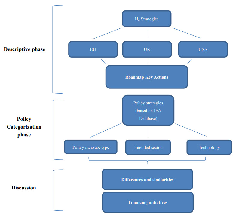
The goal of this study is twofold: first, to understand the rationales of public policies and possible outcomes on energy systems design behind supporting national hydrogen strategies in three major economic blocs (the EU, UK and USA) and possible outcomes on energy systems design; second, to identify differences in policy approaches to decarbonization through H₂ promotion. Large-scale expansion of low-carbon H₂ demands careful analysis and understanding of how public policies can be fundamental drivers of change. Our methodological approach was essentially economic, using the International Energy Agency (IEA) policy database as a main information source. First, we identified all regional policies and measures that include actions related to H₂, either directly or indirectly. Then, we reclassified policy types, sectors and technologies to conduct a comparative analysis which allowed us to reduce the high degree of economic ambiguity in the database. Finally, we composed a detailed discussion of our findings. While the EU pushed for renewable H₂, the UK immediately targeted low-carbon H₂ solutions, equally considering both blue and green alternatives. The USA pursues a clean H₂ economy based on both nuclear and CCS fossil technology. Although there is a general focus on fiscal and financing policy actions, distinct intensities were identified, and the EU presents a much stricter regulatory framework than the UK and USA. Another major difference between blocs concerns target sectors: While the EU shows a broad policy strategy, the UK is currently prioritizing the transport sector. The USA is focusing on H₂ production and supply as well as the power and heat sectors. In all cases, policy patterns and financing options seem to be in line with national hydrogen strategies, but policies' balances reflect diverse institutional frameworks and economic development models.

References

[1]	Abbas AJ, Hassani H, Burby M, et al. (2021) An investigation into the volumetric flow rate requirement of hydrogen transportation in existing natural gas pipelines and its safety implications. Gases 1: 156–179. https://doi.org/10.3390/gases1040013 doi: 10.3390/gases1040013
[2]	Abujarad SY, Mustafa MW, Jamian JJ (2017) Recent approaches of unit commitment in the presence of intermittent renewable energy resources: A review. Renew Sust Energ Rev 70: 215–223. https://doi.org/10.1016/j.rser.2016.11.246 doi: 10.1016/j.rser.2016.11.246
[3]	Acemoglu D, Aghion P, Bursztyn L, et al. (2012) The Environment and Directed Technical Change. Am Econ Rev 102: 131–166. https://doi.org/10.1257/aer.102.1.131 doi: 10.1257/aer.102.1.131
[4]	Al-Refaie A, Lepkova N (2022) Impacts of Renewable Energy Policies on CO₂ Emissions Reduction and Energy Security Using System Dynamics: The Case of Small-Scale Sector in Jordan. Sustainability 14: 5058. https://doi.org/10.3390/su14095058 doi: 10.3390/su14095058
[5]	Anderson B, Cammeraat E, Dechezleprêtre A, et al. (2021) "Policies for a climate-neutral industry: Lessons from the Netherlands", OECD Science, Technology and Industry Policy Papers, 108, OECD Publishing, Paris, Available from: https://doi.org/10.1787/a3a1f953-en.
[6]	Antenucci A, Sansavini G (2019) Extensive CO2 recycling in power systems via Power-to-Gas and network storage. Renew Sust Energ Rev 100: 33–43. https://doi.org/10.1016/j.rser.2018.10.020 doi: 10.1016/j.rser.2018.10.020
[7]	Baker F (2022) Is the United Kingdom's Hydrogen Strategy an Effective Low Carbon Strategy? Int J Energ Prod Manag 7: 164–175. https://doi.org/10.2495/EQ-V7-N2-164-175 doi: 10.2495/EQ-V7-N2-164-175
[8]	Bale CS, Varga L, Foxon TJ (2015) Energy and complexity: New ways forward. Appl Energ 138: 150–159. https://doi.org/10.1016/j.apenergy.2014.10.057 doi: 10.1016/j.apenergy.2014.10.057
[9]	Ballo A, Valentin KK, Korgo B, et al. (2022) Law and Policy Review on Green Hydrogen Potential in ECOWAS Countries. Energies 15: 2304. https://doi.org/10.3390/en15072304 doi: 10.3390/en15072304
[10]	Bersalli G, Menanteau P, El-Methni J (2020) Renewable energy policy effectiveness: A panel data analysis across Europe and Latin America. Renew Sust Energ Rev 133: 110351. https://doi.org/10.1016/j.rser.2020.110351 doi: 10.1016/j.rser.2020.110351
[11]	Bianco E, Blanco H (2020) Green hydrogen: a guide to policy making. IRENA. Available from: https://www.h2knowledgecentre.com/content/researchpaper1616.
[12]	Bölük G, Kaplan R (2022) Effectiveness of renewable energy incentives on sustainability: evidence from dynamic panel data analysis for the EU countries and Turkey. Environ Sci Pollut Res 2022: 1–18. https://doi.org/10.1007/s11356-021-17801-y doi: 10.1007/s11356-021-17801-y
[13]	Cammeraat EA, Dechezleprêtre et G Lalanne (2022) « Innovation and industrial policies for green hydrogen », OECD Science, Technology and Industry Policy Papers, n 125, Éditions OCDE, Paris. https://doi.org/10.1787/f0bb5d8c-en
[14]	Chakrabarty A (2022) UK: Applications open for first round of hydrogen funding. Sustainable Futures. Available from: https://sustainablefutures.linklaters.com/post/102htf2/uk-applications-open-for-first-round-of-hydrogen-funding.
[15]	Chen B, Xiong R, Li H, et al. (2019) Pathways for sustainable energy transition. J Clean Prod 228: 1564–1571. https://doi.org/10.1016/j.jclepro.2019.04.372 doi: 10.1016/j.jclepro.2019.04.372
[16]	Cheng W, Lee S (2022) How Green Are the National Hydrogen Strategies? Sustainability 14: 1930. https://doi.org/10.3390/su14031930 doi: 10.3390/su14031930
[17]	Chu KH, Lim J, Mang JS, et al. (2022) Evaluation of strategic directions for supply and demand of green hydrogen in South Korea. Int J Hydrogen Energ 47: 1409–1424. https://doi.org/10.1016/j.ijhydene.2021.10.107 doi: 10.1016/j.ijhydene.2021.10.107
[18]	Clean Hydrogen Partnership (2022) European Partnership for Hydrogen Technologies. Available from: https://www.clean-hydrogen.europa.eu/index_en.
[19]	Clifford C (2022) Why the EU didn't include nuclear energy in its plan to get off Russian gas. CNBC. Available from: https://www.cnbc.com/2022/03/09/why-eu-didnt-include-nuclear-energy-in-plan-to-get-off-russian-gas.html.
[20]	Côté E, Salm S (2022) Risk-adjusted preferences of utility companies and institutional investors for battery storage and green hydrogen investment. Energ Policy 163: 112821. https://doi.org/10.1016/j.enpol.2022.112821 doi: 10.1016/j.enpol.2022.112821
[21]	da Silva César A, da Silva Veras T, Mozer TS, et al. (2019) Hydrogen productive chain in Brazil: An analysis of the competitiveness' drivers. J Clean Prod 207: 751–763. https://doi.org/10.1016/j.jclepro.2018.09.157 doi: 10.1016/j.jclepro.2018.09.157
[22]	da Silva Veras T, Mozer TS, da Silva César A (2017) Hydrogen: trends, production and characterization of the main process worldwide. Int J Hydrogen Energ 42: 2018–2033. https://doi.org/10.1016/j.ijhydene.2016.08.219 doi: 10.1016/j.ijhydene.2016.08.219
[23]	de las Nieves Camacho M, Jurburg D, Tanco M (2022) Hydrogen fuel cell heavy-duty trucks: Review of main research topics. Int J Hydrogen Energ. https://doi.org/10.1016/j.ijhydene.2022.06.271 doi: 10.1016/j.ijhydene.2022.06.271
[24]	Dehhaghi S, Choobchian S, Ghobadian B, et al. (2022) Five-year development plans of renewable energy policies in Iran: a content analysis. Sustainability 14: 1501. https://doi.org/10.3390/su14031501 doi: 10.3390/su14031501
[25]	Department of Energy (DOE) (2020) Energy Department Announces Approximately $64M in Funding for 18 Projects to Advance H2@Scale. Available from: https://www.energy.gov/articles/energy-department-announces-approximately-64m-funding-18-projects-advance-h2scale.
[26]	Department of Energy (DOE) (2021) DOE Establishes New Office of Clean Energy Demonstrations Under the Bipartisan Infrastructure Law. Available from: https://www.energy.gov/articles/doe-establishes-new-office-clean-energy-demonstrations-under-bipartisan-infrastructure-law.
[27]	Department of Energy (DOE) (2022) DOE National Clean Hydrogen Strategy and Roadmap. Available from: https://www.hydrogen.energy.gov/pdfs/clean-hydrogen-strategy-roadmap.pdf.
[28]	Department of Energy² (DOE) (2021) DOE Announces $20 Million to Produce Clean Hydrogen from Nuclear Power. Available from: https://www.energy.gov/articles/doe-announces-20-million-produce-clean-hydrogen-nuclear-power.
[29]	Department of Energy² (DOE) (2022) DOE Announces Nearly $25 Million to Study Advanced Clean Hydrogen Technologies for Electricity Generation. Available from: https://www.energy.gov/articles/doe-announces-nearly-25-million-study-advanced-clean-hydrogen-technologies-electricity.
[30]	Department of Energy³ (DOE) (2021) DOE Announces $52.5 Million to Accelerate Progress in Clean Hydrogen. Available from: https://www.energy.gov/articles/doe-announces-525-million-accelerate-progress-clean-hydrogen.
[31]	Department of Energy³ (DOE) (2022) DOE Announces First Loan Guarantee for a Clean Energy Project in Nearly a Decade. Available from: https://www.energy.gov/articles/doe-announces-first-loan-guarantee-clean-energy-project-nearly-decade.
[32]	Department of Energy⁴ (DOE) (2022) DOE Announces $60 Million to Advance Clean Hydrogen Technologies and Decarbonize Grid. Available from: https://www.energy.gov/articles/doe-announces-60-million-advance-clean-hydrogen-technologies-and-decarbonize-grid.
[33]	Donoghue NM, Thompson P, Arora T (2022) UK Government Publishes Hydrogen Investment Roadmap. Available from: https://www.bakermckenzie.com/en/insight/publications/2022/04/uk-hydrogen-investment-roadmap.
[34]	Energy Efficiency and Renewable Energy (EERE) (2020) Energy Department Announces $33 Million to Advance Hydrogen and Fuel Cell R & D and the H2@Scale Vision. Available from: https://www.energy.gov/eere/articles/energy-department-announces-33-million-advance-hydrogen-and-fuel-cell-rd-and-h2scale.
[35]	Energy Efficiency and Renewable Energy (EERE) (2021) DOE Announces Nearly $8 Million for National Laboratory H2@Scale Projects to Help Reach Hydrogen Shot Goals.
[36]	Energy Efficiency and Renewable Energy (EERE) (2022) Clean Hydrogen Production Standard. Available from: https://www.energy.gov/eere/fuelcells/articles/clean-hydrogen-production-standard.
[37]	Erbach G, Jensen L (2021) EU hydrogen policy: Hydrogen as an energy carrier for a climate-neutral economy. Available from: https://policycommons.net/artifacts/1426785/eu-hydrogen-policy/2041311/.
[38]	European Commission (2019) Energy and the Green Deal: A clean energy transition. Available from: https://commission.europa.eu/strategy-and-policy/priorities-2019-2024/european-green-deal/energy-and-green-deal_en
[39]	European Commission (2020) A hydrogen strategy for a climate-neutral Europe, EPRS: European Parliamentary Research Service. Available from: https://ec.europa.eu/energy/sites/ener/files/hydrogen_strategy.pdf.
[40]	European Commission (2022) EU Emissions Trading System (EU ETS). Available from: https://ec.europa.eu/clima/eu-action/eu-emissions-trading-system-eu-ets_en.
[41]	European Commission² (2022) Key actions of the EU Hydrogen Strategy. Available from: https://energy.ec.europa.eu/topics/energy-systems-integration/hydrogen/key-actions-eu-hydrogen-strategy_en.
[42]	European Commission³ (2022) What is the Innovation Fund? Available from: https://competition-policy.ec.europa.eu/state-aid/legislation/modernisation/ipcei_en.
[43]	European Commission⁴ (2022) What is the Innovation Fund? Available from: https://climate.ec.europa.eu/eu-action/funding-climate-action/innovation-fund/what-innovation-fund_en.
[44]	European Commission⁵ (2022) REPowerEU: Joint European action for more affordable, secure and sustainable energy? Available from: https://ec.europa.eu/commission/presscorner/detail/en/ip_22_1511.
[45]	European Commission⁶ (2022) Commission awards over €1 billion to innovative projects for the EU climate transition. Available from: https://ec.europa.eu/commission/presscorner/detail/en/IP_22_2163.
[46]	European Commission⁷ (2022) EU Taxonomy Compass. Database. Available from: https://ec.europa.eu/sustainable-finance-taxonomy/home.
[47]	Falcone PM, Morone P, Sica E (2018) Greening of the financial system and fuelling a sustainability transition: A discursive approach to assess landscape pressures on the Italian financial system. Technol Forecast Soc 127: 23–37. https://doi.org/10.1016/j.techfore.2017.05.020 doi: 10.1016/j.techfore.2017.05.020
[48]	Falcone PM, Sica E (2019) Assessing the opportunities and challenges of green finance in Italy: An analysis of the biomass production sector. Sustainability 11: 517. https://doi.org/10.3390/su11020517 doi: 10.3390/su11020517
[49]	Fankhauser S, Jotzo F (2018) Economic growth and development with low‐carbon energy. Wires Clim Change 9: e495. https://doi.org/10.1002/wcc.495 doi: 10.1002/wcc.495
[50]	Faure A, Okullo SJ, Pahle M (2020) Price and quantity policies to improve the EU-ETS: which is best? Technical Report.
[51]	Fossil Energy and Carbon Management (FECM) (2022) DOE Invests $2.4 Million for Next-Generation Energy Storage Technologies. Available from: https://www.energy.gov/fecm/articles/doe-invests-24-million-next-generation-energy-storage-technologies.
[52]	Fossil Energy and Carbon Management² (FECM) (2022) U.S. Department of Energy Announces $28 Million to Develop Clean Hydrogen. Available from: https://www.energy.gov/fecm/articles/us-department-energy-announces-28-million-develop-clean-hydrogen?utm_medium = email & utm_source = govdelivery.
[53]	Gordon JA, Balta-Ozkan N, Nabavi SA (2023) Socio-technical barriers to domestic hydrogen futures: Repurposing pipelines, policies, and public perceptions. Appl Energ 336: 120850. https://doi.org/10.1016/j.apenergy.2023.120850 doi: 10.1016/j.apenergy.2023.120850
[54]	Greenstone M, Nath I (2019) Do renewable portfolio standards deliver? University of Chicago, Becker Friedman Institute for Economics Working Paper 62.
[55]	Haas R, Resch G, Panzer C, et al. (2011) Efficiency and effectiveness of promotion systems for electricity generation from renewable energy sources–Lessons from EU countries. Energy 36: 2186–2193. https://doi.org/10.1016/j.energy.2010.06.028 doi: 10.1016/j.energy.2010.06.028
[56]	Hafeznia H, Aslani A, Anwar S, et al. (2017) Analysis of the effectiveness of national renewable energy policies: A case of photovoltaic policies. Renew Sust Energ Rev 79: 669–680. https://doi.org/10.1016/j.rser.2017.05.033 doi: 10.1016/j.rser.2017.05.033
[57]	Holloway S, Vincent CJ, Kirk K (2006) Industrial carbon dioxide emissions and carbon dioxide storage potential in the UK. Nottingham, UK, British Geological Survey, 60. Available from: https://www.energy.gov/eere/articles/doe-announces-nearly-8-million-national-laboratory-h2scale-projects-help-reach.
[58]	Hoogland O, Eklund L, Dahl V (2022) The fiscal implications of the clean energy transition, Directorate-General for Energy. Publications Office of the European Union. Available from: https://data.europa.eu/doi/10.2833/941143.
[59]	Howlett M, Leong C (2022) Policy volatility and the propensity of policies to fail: dealing with uncertainty, maliciousness and compliance in public policy-making. Int J Public Policy 16: 236–252. https://doi.org/10.1504/IJPP.2022.127431 doi: 10.1504/IJPP.2022.127431
[60]	Hu J, Harmsen R, Crijns-Graus W, et al. (2018) Identifying barriers to large-scale integration of variable renewable electricity into the electricity market: A literature review of market design. Renew Sust Energ Rev 81: 2181–2195. https://doi.org/10.1016/j.rser.2017.06.028 doi: 10.1016/j.rser.2017.06.028
[61]	HyResource (2022) A collaborative knowledge sharing resource supporting the development of Australia's hydrogen industry. Available from: https://research.csiro.au/hyresource/policy/international/european-commission/.
[62]	IEA (2022) Hydrogen Projects Database. Available from: https://www.iea.org/data-and-statistics/data-product/hydrogen-projects-database.
[63]	IEA¹ (2021) Hydrogen. International Energy Agency, Paris. Available from: https://www.iea.org/reports/hydrogen.
[64]	IEA² (2021) Global Hydrogen Review 2021. IEA, Paris. Available from: https://www.iea.org/reports/global-hydrogen-review-2021.
[65]	IEA² (2022) Policies database, 2022, IEA. Available from: https://www.iea.org/policies.
[66]	IRENA (2022) World Energy Transitions Outlook 2022: 1.5℃ Pathway, International Renewable Energy Agency, Abu Dhabi.
[67]	Iribarren D, Martín-Gamboa M, Navas-Anguita Z, et al. (2020) Influence of climate change externalities on the sustainability-oriented prioritisation of prospective energy scenarios. Energy 196: 117179. https://doi.org/10.1016/j.energy.2020.117179 doi: 10.1016/j.energy.2020.117179
[68]	Jafari H, Safarzadeh S, Azad-Farsani E (2022) Effects of governmental policies on energy-efficiency improvement of hydrogen fuel cell cars: A game-theoretic approach. Energy 254: 124394. https://doi.org/10.1016/j.energy.2022.124394 doi: 10.1016/j.energy.2022.124394
[69]	Jones J, Genovese A, Tob-Ogu A (2020) Hydrogen vehicles in urban logistics: A total cost of ownership analysis and some policy implications. Renew Sust Energ Rev 119: 109595. https://doi.org/10.1016/j.rser.2019.109595 doi: 10.1016/j.rser.2019.109595
[70]	Krozer Y (2019) Financing of the global shift to renewable energy and energy efficiency. Green Financ 1: 264–278. https://doi.org/10.3934/GF.2019.3.264 doi: 10.3934/GF.2019.3.264
[71]	Kurmayer N (2021) €2 billion 'Clean Hydrogen Partnership' signals move away from hydrogen cars. Euractiv. Available from: https://www.euractiv.com/section/energy/news/e2-billion-clean-hydrogen-partnership-another-move-away-from-hydrogen-cars/.
[72]	Lezama F, Soares J, Hernandez-Leal P, et al. (2018) Local energy markets: Paving the path toward fully transactive energy systems. IEEE T Power Syst 34: 4081–4088. https://doi.org/10.1109/TPWRS.2018.2833959 doi: 10.1109/TPWRS.2018.2833959
[73]	Mahajan D, Tan K, Venkatesh T, et al. (2022) Hydrogen Blending in Gas Pipeline Networks—A Review. Energies 15: 3582. https://doi.org/10.3390/en15103582 doi: 10.3390/en15103582
[74]	Maisonneuve C (2022) European Energy Sovereignty: Putting an End to the Stigma of Nuclear Power. Institut Montaigne. Available from: https://www.institutmontaigne.org/en/blog/european-energy-sovereignty-putting-end-stigma-nuclear-power.
[75]	Marques AC, Fuinhas JA (2012) Are public policies towards renewables successful? Evidence from European countries. Renew Energ 44: 109–118. https://doi.org/10.1016/j.renene.2012.01.007 doi: 10.1016/j.renene.2012.01.007
[76]	McQueen S, Stanford J, Satyapal S, et al. (2020) Department of energy hydrogen program plan (No. DOE/EE-2128). US Department of Energy (USDOE), Washington DC (United States). https://doi.org/10.2172/1721803
[77]	Moore J, Shabani B (2016) A critical study of stationary energy storage policies in Australia in an international context: the role of hydrogen and battery technologies. Energies 9: 674. https://doi.org/10.3390/en9090674 doi: 10.3390/en9090674
[78]	OECD (2023) Economic Outlook, Interim Report March 2023: A Fragile Recovery. Available from: https://www.oecd-ilibrary.org/sites/d14d49eb-en/index.html?itemId = /content/publication/d14d49eb-en.
[79]	Oliveira AM, Beswick RR, Yan Y (2021) A green hydrogen economy for a renewable energy society. Curr Opin Chem Eng 33: 100701. https://doi.org/10.1016/j.coche.2021.100701 doi: 10.1016/j.coche.2021.100701
[80]	Park C, Lim S, Shin J, et al. (2022) How much hydrogen should be supplied in the transportation market? Focusing on hydrogen fuel cell vehicle demand in South Korea: Hydrogen demand and fuel cell vehicles in South Korea. Technol Forecast Soc Change 181: 121750. https://doi.org/10.1016/j.techfore.2022.121750 doi: 10.1016/j.techfore.2022.121750
[81]	Parkes R (2022) 'From niche to scale' \| EU launches €3bn European Hydrogen Bank with a bang but keeps quiet about the details. Recharge, 14 September 2022. Available from: https://www.rechargenews.com/energy-transition/from-niche-to-scale-eu-launches-3bn-european-hydrogen-bank-with-a-bang-but-keeps-quiet-about-the-details/2-1-1299131.
[82]	Parkes R² (2022) Biden invokes wartime legislation to ramp up US hydrogen electrolyser production, but what will this mean in practice? Available from: https://www.rechargenews.com/energy-transition/biden-invokes-wartime-legislation-to-ramp-up-us-hydrogen-electrolyser-production-but-what-will-this-mean-in-practice-/2-1-1235045.
[83]	Polzin F, Migendt M, Täube FA, et al. (2015) Public policy influence on renewable energy investments—A panel data study across OECD countries. Energ policy 80: 98-111. https://doi.org/10.1016/j.enpol.2015.01.026 doi: 10.1016/j.enpol.2015.01.026
[84]	Prăvălie R, Bandoc G (2018) Nuclear energy: Between global electricity demand, worldwide decarbonisation imperativeness, and planetary environmental implications. J Environ Manage 209: 81–92. https://doi.org/10.1016/j.jenvman.2017.12.043 doi: 10.1016/j.jenvman.2017.12.043
[85]	REPowerEU Plan (2018) Communication from the Commission to the European Parliament, the European Council, the Council, the European Economic and Social Committee and the Committee of the Regions.
[86]	Rodríguez MLÁ, Flores JJA, Vera JVA, et al. (2022) The regulatory framework of the hydrogen market in Mexico: a look at energy governance. Int J Hydrogen Energ 47: 29986–29998. https://doi.org/10.1016/j.ijhydene.2022.05.168 doi: 10.1016/j.ijhydene.2022.05.168
[87]	Roy J, Ghosh D, Ghosh A, et al. (2013) Fiscal instruments: crucial role in financing low carbon transition in energy systems. Curr Opin Environ Sust 5: 261–269. https://doi.org/10.1016/j.cosust.2013.05.003 doi: 10.1016/j.cosust.2013.05.003
[88]	S & P Global Commodity insights (2022) UK's gas grid ready for 20% hydrogen blend from 2023: network companies. Electric Power. Energy Transition. Natural Gas. Available from: https://www.spglobal.com/commodityinsights/en/market-insights/latest-news/electric-power/011422-uks-gas-grid-ready-for-20-hydrogen-blend-from-2023-network-companies.
[89]	Sasanpour S, Cao KK, Gils HC, et al. (2021) Strategic policy targets and the contribution of hydrogen in a 100% renewable European power system. Energ Rep 7: 4595–4608. https://doi.org/10.1016/j.egyr.2021.07.005 doi: 10.1016/j.egyr.2021.07.005
[90]	Shin J, Hwang WS, Choi H (2019) Can hydrogen fuel vehicles be a sustainable alternative on vehicle market? Comparison of electric and hydrogen fuel cell vehicles. Technol Forecast Soc 143: 239–248. https://doi.org/10.1016/j.techfore.2019.02.001 doi: 10.1016/j.techfore.2019.02.001
[91]	Surana K, Anadon LD (2015) Public policy and financial resource mobilization for wind energy in developing countries: A comparison of approaches and outcomes in China and IndiaGlob. Environ. Chang, 35: 340–359. https://doi.org/10.1016/j.gloenvcha.2015.10.001
[92]	Talebian H, Herrera OE, Mérida W (2021) Policy effectiveness on emissions and cost reduction for hydrogen supply chains: The case for British Columbia. Int J Hydrogen Energ 46: 998–1011. https://doi.org/10.1016/j.ijhydene.2020.09.190 doi: 10.1016/j.ijhydene.2020.09.190
[93]	UK Government (2020) The ten point plan for a green industrial revolution. Department for Business, Energy & Industrial Strategy. Available from: https://www.gov.uk/government/publications/the-ten-point-plan-for-a-green-industrial-revolution.
[94]	UK Government (2021) UK Hydrogen Strategy. Department for Business, Energy & Industrial Strategy. Available from: https://www.gov.uk/government/publications/the-ten-point-plan-for-a-green-industrial-revolution.
[95]	UK Government (2022) Hydrogen Strategy update to the market: July 2022. Department for Business Energy & Industrial Strategy. Available from: https://assets.publishing.service.gov.uk/government/uploads/system/uploads/attachment_data/file/1092555/hydrogen-strategy-update-to-the-market-july-2022.pdf.
[96]	UK Government² (2021) Net Zero Strategy: Build Back Greener. Available from: https://www.gov.uk/government/publications/net-zero-strategy.
[97]	UK Government² (2022) Hydrogen BECCS Innovation Programme: successful projects. Available from: https://www.gov.uk/government/publications/hydrogen-beccs-innovation-programme-successful-projects.
[98]	UK Government³ (2021) Industrial Fuel Switching competition Phase 1: feasibility studies. Available from: https://www.gov.uk/government/publications/industrial-fuel-switching-competition.
[99]	UK Government³ (2022) Government unveils investment for energy technologies of the future. Available from: https://www.gov.uk/government/news/government-unveils-investment-for-energy-technologies-of-the-future.
[100]	UK Government⁴ (2021) Tees Valley multi-modal hydrogen transport hub. Available from: https://www.gov.uk/government/publications/tees-valley-multi-modal-hydrogen-transport-hub.
[101]	UK Government⁴ (2022) UK Low Carbon Hydrogen Standard: emissions reporting and sustainability criteria. Available from: https://www.gov.uk/government/publications/uk-low-carbon-hydrogen-standard-emissions-reporting-and-sustainability-criteria.
[102]	UK Government⁵ (2021) Rail centre and green energy funding in Budget boost for Wales. Available from: https://www.gov.uk/government/news/rail-centre-and-green-energy-funding-in-budget-boost-for-wales.
[103]	Van de Graaf T, Overland I, Scholten D, et al. (2020) The new oil? The geopolitics and international governance of hydrogen. Energ Res Soc Sci 70: 101667. https://doi.org/10.1016/j.erss.2020.101667 doi: 10.1016/j.erss.2020.101667
[104]	Van Renssen S (2020) The hydrogen solution? Nat Clim Change 10: 799–801. https://doi.org/10.1038/s41558-020-0891-0 doi: 10.1038/s41558-020-0891-0
[105]	Willner M, Perino G (2022) Beyond control: Policy incoherence of the EU emissions trading system. Politics Gov10: 256–264. https://doi.org/10.17645/pag.v10i1.4797 doi: 10.17645/pag.v10i2.5183
[106]	Ye F, Paulson N, Khanna M (2022) Are renewable energy policies effective to promote technological change? The role of induced technological risk. J Environ Econ Manag 114: 102665. https://doi.org/10.1016/j.jeem.2022.102665 doi: 10.1016/j.jeem.2022.102665
[107]	Zahedi R, Zahedi A, Ahmadi A (2022) Strategic study for renewable energy policy, optimizations and sustainability in Iran. Sustainability 14: 2418. https://doi.org/10.3390/su14042418 doi: 10.3390/su14042418

GF-05-02-011-s001.pdf

Reader Comments

Your name:*

Email:*
© 2023 the Author(s), licensee AIMS Press. This is an open access article distributed under the terms of the Creative Commons Attribution License (http://creativecommons.org/licenses/by/4.0)