Does corporate reputation play a mediating role in the association between manufacturing companies' corporate social responsibility (CSR) and financial performance?

Zhang Jing; Gazi Md. Shakhawat Hossain; Badiuzzaman; Md. Shahinur Rahman; Najmul Hasan; Zhang Jing; Gazi Md. Shakhawat Hossain; Badiuzzaman; Md. Shahinur Rahman; Najmul Hasan

doi:10.3934/GF.2023010

Green Finance

2023, Volume 5, Issue 2: 240-264. doi: 10.3934/GF.2023010

Previous Article Next Article

Research article

Does corporate reputation play a mediating role in the association between manufacturing companies' corporate social responsibility (CSR) and financial performance?

1.
School of Management (SoM), Huazhong University of Science and Technology (HUST), 1037 Luoyu Road, Wuhan, Hubei 430074, China
2.
Department of Business Administration, Faculty of Business and Economics, University of Global Village (UGV), Barishal-8200, Bangladesh
3.
Department of Economics and Sociology, Faculty of Business Administration, Patuakhali Science and Technology University (PSTU), Dumki-8602, Patuakhali, Bangladesh
4.
Department of Business Administration, School of Business, Northern University of Business and Technology (NUBT), Sonadanga-9100, Khulna, Bangladesh
5.
Department of Information Systems, BRAC Business School, BRAC University, Mohakhali, Dhaka-1212, Bangladesh

Received: 13 April 2023 Revised: 19 June 2023 Accepted: 20 June 2023 Published: 27 June 2023
JEL Codes: G19, L60, M10, M14, O14

The main objective of this research was to analyze the variable of corporate reputation as a mediating variable to determine the relationship between corporate social responsibility and financial performance. Simple random sampling was used in the study to obtain 300 respondents from Bangladeshi manufacturing companies. Statistical Package for the Social Sciences (SPSS) 23.0 was used to analyze the data. To evaluate the hypotheses in this study, structural equation modeling (SEM) was used. The results demonstrated that corporate social responsibility positively influences corporate reputation and financial performance, while corporate reputation is statistically significant for financial performance. Environmental contribution, philanthropic responsibility, legal responsibility, ethical responsibility, economic responsibility and social responsibility are listed in order of significance as corporate social responsibility factors. It was determined how corporate reputation influences the link between corporate social responsibility and financial performance. However, it may be logical to conclude that there is a considerable correlation between corporate social responsibility and financial performance based on the data analysis. The results of corporate social responsibility practices in manufacturing organizations in developing nations, particularly Bangladesh, have significant consequences for businesses, entrepreneurs, communities, researchers and policymakers in understanding the outcomes of sustainability. The conclusion has drawn implications for sustainability practice and future research.
- corporate social responsibility (CSR),
- financial performance (FP),
- manufacturing firm (MF),
- corporate reputation (CR)
Citation: Zhang Jing, Gazi Md. Shakhawat Hossain, Badiuzzaman, Md. Shahinur Rahman, Najmul Hasan. Does corporate reputation play a mediating role in the association between manufacturing companies' corporate social responsibility (CSR) and financial performance?[J]. Green Finance, 2023, 5(2): 240-264. doi: 10.3934/GF.2023010

Related Papers:

Abstract

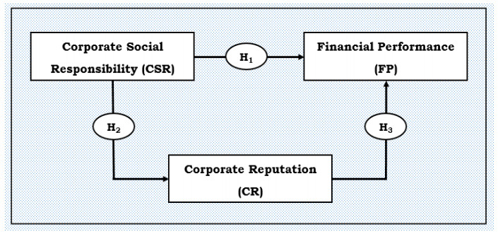
The main objective of this research was to analyze the variable of corporate reputation as a mediating variable to determine the relationship between corporate social responsibility and financial performance. Simple random sampling was used in the study to obtain 300 respondents from Bangladeshi manufacturing companies. Statistical Package for the Social Sciences (SPSS) 23.0 was used to analyze the data. To evaluate the hypotheses in this study, structural equation modeling (SEM) was used. The results demonstrated that corporate social responsibility positively influences corporate reputation and financial performance, while corporate reputation is statistically significant for financial performance. Environmental contribution, philanthropic responsibility, legal responsibility, ethical responsibility, economic responsibility and social responsibility are listed in order of significance as corporate social responsibility factors. It was determined how corporate reputation influences the link between corporate social responsibility and financial performance. However, it may be logical to conclude that there is a considerable correlation between corporate social responsibility and financial performance based on the data analysis. The results of corporate social responsibility practices in manufacturing organizations in developing nations, particularly Bangladesh, have significant consequences for businesses, entrepreneurs, communities, researchers and policymakers in understanding the outcomes of sustainability. The conclusion has drawn implications for sustainability practice and future research.

References

[1]	Abu-Baker N, Naser K (2000). Empirical evidence on corporate social disclosure (CSD) practices in Jordan. Int J Commer Manage 10: 18–34. https://doi.org/10.1108/eb047406
[2]	Adamkaite J, Streimikiene D, Rudzioniene K (2023) The impact of social responsibility on corporate financial performance in the energy sector: Evidence from Lithuania. Corp Soc Resp Envir Ma. https://doi.org/10.1002/csr.2340
[3]	Aggarwal A, Saxena N (2023) Examining the relationship between corporate social responsibility, corporate reputation and brand equity in Indian banking industry. J Public Aff 23: e2838. https://doi.org/10.1002/pa.2838
[4]	Aguilera RV, Rupp DE, Williams CA, et al. (2022) Organizational governance and ethics: An ongoing research agenda. J Bus Ethics 183: 529–546.
[5]	Ahamed WSW, Almsafir MK, Al-Smadi AW (2014) Does corporate social responsibility lead to improve in firm financial performance? Evidence from Malaysia. Int J Econ Financ 6: 126–138. https://doi.org/10.5539/ijef.v6n3p126 doi: 10.5539/ijef.v6n3p126
[6]	AlAjmi J, Buallay A, Saudagaran S (2023) Corporate social responsibility disclosure and banks' performance: the role of economic performance and institutional quality. Int J Soc Econ 50: 359–376. https://doi.org/10.1108/IJSE-11-2020-0757 doi: 10.1108/IJSE-11-2020-0757
[7]	Alarcón D, Sánchez JA, De Olavide U (2015) Assessing convergent and discriminant validity in the ADHD-R IV rating scale: User-written commands for Average Variance Extracted (AVE), Composite Reliability (CR), and Heterotrait-Monotrait ratio of correlations (HTMT). In Spanish STATA Meeting, 1–39.
[8]	Ali HY, Danish RQ, Asrar-ul-Haq M (2020) How corporate social responsibility boosts firm financial performance: The mediating role of corporate image and customer satisfaction. Corp Soc Resp Environ Ma 27: 166–177. https://doi.org/10.1002/csr.1781 doi: 10.1002/csr.1781
[9]	Al-Sfan MBB (2023) A Study of the Relationship Between Social Responsibility and Earning Management And Its Reflection On The Financial Performance Of A Sample Of Companies Listed On The Iraq Stock Exchange. World Bull Manage Law18: 8–18.
[10]	Amran A, Siti-Nabiha A (2009) Corporate social reporting in Malaysia: a case of mimicking the West or succumbing to local pressure. Soc Resp J. https://doi.org/10.1108/17471110910977285
[11]	Aranguren Gómez N, Maldonado García S (2022) Building Corporate Reputation Through Corporate Social Responsibility Disclosures. The Case of Colombian Companies. Corp Rep Rev, 1–25. https://doi.org/10.1057/s41299-022-00155-7
[12]	Aupperle KE, Van Pham D (1989) An expanded investigation into the relationship of corporate social responsibility and financial performance. Employ Responsib Rig J 2: 263–274. https://doi.org/10.1007/BF01423356 doi: 10.1007/BF01423356
[13]	Azzalini A, Browne RP, Genton MG, et al. (2016) On nomenclature for, and the relative merits of, two formulations of skew distributions. Stat Prob Lett 110: 201–206. https://doi.org/10.1016/j.spl.2015.12.008 doi: 10.1016/j.spl.2015.12.008
[14]	Babalola YA (2012) The impact of corporate social responsibility on firms' profitability in Nigeria. Eur J Econ Financ Adm Sci 45: 39–50.
[15]	Bagozzi RP, Yi Y, Phillips LW (1991) Assessing construct validity in organizational research. Adm Sci Q, 421–458. https://doi.org/10.2307/2393203 doi: 10.2307/2393203
[16]	Baldarelli MG, Gigli S (2014) Exploring the drivers of corporate reputation integrated with a corporate responsibility perspective: some reflections in theory and in praxis. J Manage Gov 18: 589–613. https://doi.org/10.1007/s10997-011-9192-3 doi: 10.1007/s10997-011-9192-3
[17]	Balmer JM, Powell SM, Hildebrand D, et al. (2011) Corporate social responsibility: a corporate marketing perspective. Eur J Mark. https://doi.org/10.1108/03090561111151790 doi: 10.1108/03090561111151790
[18]	Barnett ML (2007) Stakeholder influence capacity and the variability of financial returns to corporate social responsibility. Acade Manage Rev 32: 794–816. https://doi.org/10.5465/amr.2007.25275520 doi: 10.5465/amr.2007.25275520
[19]	Barnett ML, Jermier JM, Lafferty BA (2006) Corporate reputation: The definitional landscape. Corp Rep Rev 9: 26–38. https://doi.org/10.1057/palgrave.crr.1550012 doi: 10.1057/palgrave.crr.1550012
[20]	Baron RM, Kenny DA (1986) The moderator–mediator variable distinction in social psychological research: Conceptual, strategic, and statistical considerations. J Pers Soc Psy 51: 1173. https://doi.org/10.1037/0022-3514.51.6.1173
[21]	Bashir M (2022) Corporate social responsibility and financial performance–the role of corporate reputation, advertising and competition. PSU Res Rev. https://doi.org/10.1108/PRR-10-2021-0059
[22]	Bebbington J, Larrinaga-González C, Moneva-Abadía JM (2008) Legitimating reputation/the reputation of legitimacy theory. Account Audit Account J. https://doi.org/10.1108/09513570810863969
[23]	Becerra-Vicario R, Ruiz-Palomo D, León-Gómez A, et al. (2023) The Relationship between Innovation and the Performance of Small and Medium-Sized Businesses in the Industrial Sector: The Mediating Role of CSR. Economies 11: 92. https://doi.org/10.3390/economies11030092
[24]	Belal AR (2001) A study of corporate social disclosures in Bangladesh. Manag Audit J.
[25]	Black BS, Khanna VS (2007) Can corporate governance reforms increase firm market values? Event study evidence from India. J Empir Legal Stud 4: 749–796. https://doi.org/10.1111/j.1740-1461.2007.00106.x doi: 10.1111/j.1740-1461.2007.00106.x
[26]	Boyle EJ, Higgins MM, Rhee GS (1997) Stock market reaction to ethical initiatives of defense contractors: Theory and evidence. Crit Perspect Accoun 8: 541–561. https://doi.org/10.1006/cpac.1997.0124 doi: 10.1006/cpac.1997.0124
[27]	Brinkmann F, Gerstmeier E, Schiereck D (2020) Community engagement and corporate social responsibility (CSR): An overview and recent developments. J Bus Ethics 161: 1–21.
[28]	Bromley DB (2000) Psychological aspects of corporate identity, image and reputation. Corp Rep Rev 3: 240–252. https://doi.org/10.1057/palgrave.crr.1540117 doi: 10.1057/palgrave.crr.1540117
[29]	Cabrera-Luján SL, Sánchez-Lima DJ, Guevara-Flores SA, et al. (2023) Impact of Corporate Social Responsibility, Business Ethics and Corporate Reputation on the Retention of Users of Third-Sector Institutions. Sustainability 15: 1781. https://doi.org/10.3390/su15031781
[30]	Carroll AB (1979) A three-dimensional conceptual model of corporate performance. Acad Manage Rev 4: 497–505. https://doi.org/10.2307/257850 doi: 10.2307/257850
[31]	Carroll AB, Shabana KM (2021) The business case for corporate social responsibility: A review of concepts, research, and practice. Oxf Res Encyclopedia Bus Manage.
[32]	Chen P (2023) Corporate social responsibility, financing constraints, and corporate carbon intensity: new evidence from listed Chinese companies. Environ Sci Pollut Res, 1–9. https://doi.org/10.1007/s11356-023-25176-5
[33]	Chen Y, Xu Z, Wang X, et al. (2023) How does green credit policy improve corporate social responsibility in China? An analysis based on carbon-intensive listed firms. Corp Soc Resp Environ Manage 30: 889–904. https://doi.org/10.1002/csr.2395 doi: 10.1002/csr.2395
[34]	Cheng B, Ioannou I, Serafeim G (2014) Corporate social responsibility and access to finance. Strat Manage J 35: 1–23. https://doi.org/10.1002/smj.2131 doi: 10.1002/smj.2131
[35]	Chih C (2023) The impact of perceived corporate social responsibility on participating in philanthropic road-running events: a moderated mediation model. Sport Bus Manage Int J. https://doi.org/10.1108/SBM-05-2022-0038
[36]	Chung KH, Yu JE, Choi MG, et al. (2015) The effects of CSR on customer satisfaction and loyalty in China: the moderating role of corporate image. J Econ Bus Manage 3: 542–547. https://doi.org/10.7763/JOEBM.2015.V3.243 doi: 10.7763/JOEBM.2015.V3.243
[37]	Cochran PL, Wood RA (1984) Corporate social responsibility and financial performance. Acad Manage J 27: 42–56. https://doi.org/10.2307/255956 doi: 10.2307/255956
[38]	Cox BJ, Fleet C, Stein MB (2004) Self-criticism and social phobia in the US national comorbidity survey. J Affect Disorders 82: 227–234. https://doi.org/10.1016/j.jad.2003.12.012 doi: 10.1016/j.jad.2003.12.012
[39]	Das KP, Mukhopadhyay S, Suar D (2023) Enablers of workforce agility, firm performance, and corporate reputation. Asia Pacific Manage Rev 28: 33–44. https://doi.org/10.1016/j.apmrv.2022.01.006 doi: 10.1016/j.apmrv.2022.01.006
[40]	Dentchev NA (2004) Corporate social performance as a business strategy. J Bus Ethics 55: 395–410. https://doi.org/10.1007/s10551-004-1348-5
[41]	Dobers P, Halme M (2009) Corporate social responsibility and developing countries. Corp Soc Resp Environ Manage 16: 237–249. https://doi.org/10.1002/csr.212 doi: 10.1002/csr.212
[42]	Donaldson T, Preston LE (1995) The stakeholder theory of the corporation: Concepts, evidence, and implications. Acad ManageRev 20: 65–91. https://doi.org/10.2307/258887 doi: 10.2307/258887
[43]	Dwertmann DJ, Goštautaitė B, Kazlauskaitė R, et al. (2023) Receiving service from a person with a disability: Stereotypes, perceptions of corporate social responsibility, and the opportunity for increased corporate reputation. Acad Manage J 66: 133–163. https://doi.org/10.5465/amj.2020.0084 doi: 10.5465/amj.2020.0084
[44]	Eberl M, Schwaiger M (2005) Corporate reputation: disentangling the effects on financial performance. Eur J Mark. https://doi.org/10.1108/03090560510601798
[45]	Farooq SU, Ullah S, Kimani D (2015) The Relationship between Corporate Governance and Corporate Social Responsibility (CSR) Disclosure: Evidence from the USA. Abasyn Univ J Soc Sci 8.
[46]	Fauzi H, Idris K (2009) The relationship of CSR and financial performance: New evidence from Indonesian companies. Issues Soc Enviro Account 3. https://doi.org/10.22164/isea.v3i1.38
[47]	Fauzi H, Mahoney LS, Abdul Rahman A (2007) Institutional ownership and corporate social performance: Empirical evidence from Indonesian companies. Issues Soc Environ Account 1: 334–347. https://doi.org/10.22164/isea.v1i2.21 doi: 10.22164/isea.v1i2.21
[48]	Febra L, Costa M, Pereira F (2023) Reputation, return and risk: A new approach. Eur Res Manage Bus Econ 29: 100207. https://doi.org/10.1016/j.iedeen.2022.100207
[49]	Fombrun CJ, Rindova V (1996) Who's tops and who decides? The social construction of corporate reputations. New York University, Stern School of Business, Working Paper, 5–13.
[50]	Fornell C, Larcker DF (1981) Structural equation models with unobservable variables and measurement error: Algebra and statistics. https://doi.org/10.2307/3150980
[51]	Frerichs IM, Teichert T (2023) Research streams in corporate social responsibility literature: a bibliometric analysis. Manage Rev Q 73: 231–261. https://doi.org/10.1007/s11301-021-00237-6 doi: 10.1007/s11301-021-00237-6
[52]	Friedman AL, Miles S (2001) Socially responsible investment and corporate social and environmental reporting in the UK: an exploratory study. Brit Account Rev 33: 523–548. https://doi.org/10.1006/bare.2001.0172 doi: 10.1006/bare.2001.0172
[53]	Frooman J (1997) Socially irresponsible and illegal behavior and shareholder wealth: A meta-analysis of event studies. Bus Soc 36: 221–249. https://doi.org/10.1177/000765039703600302 doi: 10.1177/000765039703600302
[54]	Galbreath J, Shum P (2012) Do customer satisfaction and reputation mediate the CSR–FP link? Evidence from Australia. Aust J Manage 37: 211–229. https://doi.org/10.1177/0312896211432941 doi: 10.1177/0312896211432941
[55]	García-Rosell JC, Moisander J, Mäkinen J (2023) Conceptual framework for understanding the ethical dimension of corporate social responsibility, New Directions in Art, Fashion, and Wine: Sustainability, Digitalization, and Artification, 139.
[56]	Ghardallou W (2022) Corporate sustainability and firm performance: the moderating role of CEO education and tenure. Sustainability 14: 3513. https://doi.org/10.3390/su14063513
[57]	Gimeno-Arias F, Santos-Jaén JM, Palacios-Manzano M, et al. (2021) Using PLS-SEM to analyze the effect of CSR on corporate performance: The mediating role of human resources management and customer satisfaction. An empirical study in the Spanish food and beverage manufacturing sector. Mathematics 9: 2973. https://doi.org/10.3390/math9222973
[58]	Godfrey PC (2005) The relationship between corporate philanthropy and shareholder wealth: A risk management perspective. Acad Manage Rev 30: 777–798. https://doi.org/10.5465/amr.2005.18378878 doi: 10.5465/amr.2005.18378878
[59]	Goi CL, Yong KH (2009) Contribution of public relations (PR) to corporate social responsibility (CSR): A review on Malaysia perspective. Int J Mark Stud 1: 46. https://doi.org/10.5539/ijms.v1n2p46
[60]	Graafland J, Mazereeuw-Van der Duijn Schouten C (2012) Motives for corporate social responsibility. De Economist 160: 377–396. https://doi.org/10.1007/s10645-012-9198-5 doi: 10.1007/s10645-012-9198-5
[61]	Greening DW, Turban DB (2000) Corporate social performance as a competitive advantage in attracting a quality workforce. Bus Soc 39: 254–280. https://doi.org/10.1177/000765030003900302 doi: 10.1177/000765030003900302
[62]	Hair JF, Sarstedt M, Ringle CM, et al. (2012) An assessment of the use of partial least squares structural equation modeling in marketing research. J Acad Mark Sci 40: 414–433. https://doi.org/10.1007/s11747-011-0261-6 doi: 10.1007/s11747-011-0261-6
[63]	Handayani R, Wahyudi S, Suharnomo S (2017) The effects of corporate social responsibility on manufacturing industry performance: the mediating role of social collaboration and green innovation. Bus Theory Pract 18: 152–159. https://doi.org/10.3846/btp.2017.016 doi: 10.3846/btp.2017.016
[64]	Helm S (2007) The role of corporate reputation in determining investor satisfaction and loyalty. Corp Rep Rev 10: 22–37. https://doi.org/10.1057/palgrave.crr.1550036 doi: 10.1057/palgrave.crr.1550036
[65]	Hill A, Roberts J, Ewings P, et al. (1997) Non-response bias in a lifestyle survey. J Public Health 19: 203–207. https://doi.org/10.1093/oxfordjournals.pubmed.a024610 doi: 10.1093/oxfordjournals.pubmed.a024610
[66]	Hossain GMS, Rahman MS, Das S (2019) A Structural Equation Modeling (SEM) Approach to Explore the Association between Corporate Social Responsibility and Financial Performance: A Single Mediating Mechanism. North Am Acad Res 2: 155–172.
[67]	Hur WM, Kim H, Woo J (2014) How CSR leads to corporate brand equity: Mediating mechanisms of corporate brand credibility and reputation. J Bus Ethics 125: 75–86. https://doi.org/10.1007/s10551-013-1910-0 doi: 10.1007/s10551-013-1910-0
[68]	Hutton W, MacDougall A, Zadek S (2001) Session 3: Topics in Business Ethics: Corporate Stakeholding, Ethical Investment, Social Acconting. J Bus Ethics, 107–117. https://doi.org/10.1023/A:1010641830759 doi: 10.1023/A:1010641830759
[69]	Imam S (2000) Corporate social performance reporting in Bangladesh. Manage Audit J. https://doi.org/10.1108/02686900010319384
[70]	Ingram RW, Frazier KB (1980) Environmental performance and corporate disclosure. J Account Res, 614–622. https://doi.org/10.2307/2490597
[71]	Iqbal N, Ahmad N, Basheer NA, et al. (2012) Impact of corporate social responsibility on financial performance of corporations: Evidence from Pakistan. Int J Learn Dev 2: 107–118. https://doi.org/10.5296/ijld.v2i6.2717 doi: 10.5296/ijld.v2i6.2717
[72]	Islam ZM, Ahmed SU, Hasan I (2012) Corporate social responsibility and financial performance linkage: Evidence from the banking sector of Bangladesh. J Organ Manage 1: 14–21. https://doi.org/10.1002/csr.1298 doi: 10.1002/csr.1298
[73]	Javed M, Rashid MA, Hussain G, et al. (2020) The effects of corporate social responsibility on corporate reputation and firm financial performance: Moderating role of responsible leadership. Corp Soc Resp Environ Manage 27: 1395–1409. https://doi.org/10.1002/csr.1892 doi: 10.1002/csr.1892
[74]	Jiang H, Cheng Y, Park K, et al. (2022) Linking CSR communication to corporate reputation: Understanding hypocrisy, employees' social media engagement and CSR-related work engagement. Sustainability 14: 2359. https://doi.org/10.3390/su14042359
[75]	Johnson RA, Greening DW (1999) The effects of corporate governance and institutional ownership types on corporate social performance. Acad Manage J 42: 564–576. https://doi.org/10.2307/256977 doi: 10.2307/256977
[76]	Julian SD, Ofori-dankwa JC (2013) Financial resource availability and corporate social responsibility expenditures in a sub-Saharan economy: The institutional difference hypothesis. Strat Manage J 34: 1314–1330. https://doi.org/10.1002/smj.2070 doi: 10.1002/smj.2070
[77]	Khan HUZ (2010) The effect of corporate governance elements on corporate social responsibility (CSR) reporting: Empirical evidence from private commercial banks of Bangladesh. Int J Law Manage 52: 82–109. https://doi.org/10.1108/17542431011029406 doi: 10.1108/17542431011029406
[78]	Kiliç M, Kuzey C, Uyar A (2015) The impact of ownership and board structure on Corporate Social Responsibility (CSR) reporting in the Turkish banking industry. Corp Gov. https://doi.org/10.1108/CG-02-2014-0022
[79]	Kim RC (2022) Rethinking corporate social responsibility under contemporary capitalism: Five ways to reinvent CSR. Bus Ethics Environ Respon 31: 346–362. https://doi.org/10.1111/beer.12414 doi: 10.1111/beer.12414
[80]	Kusakci S, Bushera I (2023) Corporate social responsibility pyramid in Ethiopia: A mixed study on approaches and practices. Int J Bus Ecosyst Strat (2687–2293) 5: 37–48. https://doi.org/10.36096/ijbes.v5i1.378
[81]	Le TT (2022) Corporate social responsibility and SMEs' performance: mediating role of corporate image, corporate reputation and customer loyalty. Int J Emerg Mark. https://doi.org/10.1108/IJOEM-07-2021-1164
[82]	Lee KH, Herold DM, Yu AL (2016) Small and medium enterprises and corporate social responsibility practice: A Swedish perspective. Corp Soc Respon Environ Manage 23: 88–99. https://doi.org/10.1002/csr.1366 doi: 10.1002/csr.1366
[83]	Leong LY, Hew TS, Ooi KB, et al. (2012) The determinants of customer loyalty in Malaysian mobile telecommunication services: a structural analysis. Int J Serv Econ Manage 4: 209–236. https://doi.org/10.1504/IJSEM.2012.048620 doi: 10.1504/IJSEM.2012.048620
[84]	León-Gómez A, Santos-Jaén JM, Ruiz-Palomo D, et al. (2022) Disentangling the impact of ICT adoption on SMEs performance: the mediating roles of corporate social responsibility and innovation. Oeconomia Copernicana 13: 831–866. https://doi.org/10.24136/oc.2022.024 doi: 10.24136/oc.2022.024
[85]	Li J, Fu T, Han S, et al. (2023) Exploring the Impact of Corporate Social Responsibility on Financial Performance: The Moderating Role of Media Attention. Sustainability 15: 5023. https://doi.org/10.3390/su15065023
[86]	Little PL, Little BL (2000) Do perceptions of corporate social responsibility contribute to explaining differences in corporate price-earnings ratios? A research note. Corp Reput Rev 3: 137–142. https://doi.org/10.1057/palgrave.crr.1540108 doi: 10.1057/palgrave.crr.1540108
[87]	Liu X, Vredenburg H, Steel P (2019) Exploring the mechanisms of corporate reputation and financial performance: A meta-analysis. Acad Manage Proc 2019: 17903. https://doi.org/10.5465/AMBPP.2019.193
[88]	Low MP (2016) Corporate social responsibility and the evolution of internal corporate social responsibility in 21st century. Asian J Soc Sci Manage Stud 3: 56–74. https://doi.org/10.20448/journal.500/2016.3.1/500.1.56.74 doi: 10.20448/journal.500/2016.3.1/500.1.56.74
[89]	Lynch-Wood G, Williamson D, Jenkins W (2009) The over-reliance on self-regulation in CSR policy. Bus Ethics Eur Rev 18: 52–65. https://doi.org/10.1111/j.1467-8608.2009.01548.x doi: 10.1111/j.1467-8608.2009.01548.x
[90]	Maalim BM, Kibe LW, Ndolo J (2023) Assessment of Shareholder Strategy–An Internal Corporate Social Responsibility Perspective on Organizational Commitment in Five-Star Hotels in Kenya. Asian J Econ Bus Account 23: 72–85. https://doi.org/10.9734/ajeba/2023/v23i141006 doi: 10.9734/ajeba/2023/v23i141006
[91]	Madueno JH, Jorge ML, Conesa IM, et al. (2016) Relationship between corporate social responsibility and competitive performance in Spanish SMEs: Empirical evidence from a stakeholders' perspective. BRQ Bus Res Q 19: 55–72. https://doi.org/10.1016/j.brq.2015.06.002 doi: 10.1016/j.brq.2015.06.002
[92]	Maignan I (2001) Consumers' perceptions of corporate social responsibilities: A cross-cultural comparison. J Bus Ethics 30: 57–72. https://doi.org/10.1023/A:1006433928640 doi: 10.1023/A:1006433928640
[93]	Maignan I, Ferrell OC (2000) Measuring corporate citizenship in two countries: The case of the United States and France. J Bus Ethics 23: 283–297. https://doi.org/10.1023/A:1006262325211 doi: 10.1023/A:1006262325211
[94]	Maignan I, Ferrell OC, Hult GTM (1999) Corporate citizenship: Cultural antecedents and business benefits. J Acad Mark Sci 27: 455–469. https://doi.org/10.1177/0092070399274005 doi: 10.1177/0092070399274005
[95]	Mankelow G, Quazi A (2007) Factors affecting SMEs motivations for corporate social responsibility. In 3Rs: Reputation, Responsibility & Relevance: Australian and New Zealand Marketing Academy (ANZMAC) Conference 2007 (ANZMAC 2007), Australian and New Zealand Marketing Academy, 2367–2374.
[96]	Masud AA, Hossain GMS (2019) A Model to Explain How an Organization's Corporate Social Responsibility (CSR) Contributes to Corporate Image and Financial Performance: By Using Structural Equation Modelling (SEM). Int J Manage IT Eng 9: 32–52.
[97]	Masud A, Hoque AAM, Hossain MS, et al. (2013) Corporate social responsibility practices in garments sector of bangladesh, A study of multinational garments, CSR view in dhaka EPZ. Dev Country Stud 3: 27–37.
[98]	Masud AA (2018) Corporate Social Responsibility and Customer Loyalty, How Corporate Social Responsibility lead to Firm Performance: A Study on textile sector in Southern Bangladesh. Barisal UnivJ J Bus Stud 4: 180–192.
[99]	Masud AA, Ferdous R (2016) Relationship between the Expenditure of Corporate Social Responsibility and the Export Growth of Readymade Garments Sector; An Econometric Review based on Bangladesh perspective. J Bus Res Publicat Bus Res Bureau 1: 23–44.
[100]	Masud AA, Islam S (2018) The relationship between corporate social responsibility (CSR) and financial performance of textiles sector in Bangladesh especially in Barisal Division. Int J Adv Soc Sci Human 5: 6–16.
[101]	Masud AA, Ferdous R, Hossain DMM (2017) Corporate Social responsibility practices on the productivity of readymade garments sector in Bangladesh. Barisal Uni J J Art Human Soc Sci Law 1: 5–18.
[102]	McGee JE (2021) Nonfinancial disclosure and its impact on sustainability, social responsibility, and ethics research. J Bus Ethics 169: 1–21.
[103]	McWilliams A, Siegel D (2000) Corporate social responsibility and financial performance: correlation or misspecification? Strat Manage J 21: 603–609. https://doi.org/10.1002/(SICI)1097-0266(200005)21:5<603::AID-SMJ101>3.0.CO;2-3 doi: 10.1002/(SICI)1097-0266(200005)21:5<603::AID-SMJ101>3.0.CO;2-3
[104]	McWilliams A, Siegel D (2001) Corporate social responsibility: A theory of the firm perspective. Acade Manage Rev 26: 117–127. https://doi.org/10.2307/259398 doi: 10.2307/259398
[105]	Mishra S, Suar D (2010) Does corporate social responsibility influence firm performance of Indian companies? J Bus Ethics 95: 571–601. https://doi.org/10.1007/s10551-010-0441-1 doi: 10.1007/s10551-010-0441-1
[106]	Mitnick BM, Windsor D, Wood DJ (2023) Moral CSR. Bus Soc 62: 192–220. https://doi.org/10.1177/00076503221086881 doi: 10.1177/00076503221086881
[107]	, Abdullah KH, Mohd-Sabrun I (2023) Research on corporate reputation: A bibliometric review of 43 years (1977−2020). Int J Infor Scienc Manage (IJISM) 21: 31–54.
[108]	Moore G, Spence L (2006) Responsibility and small business. https://doi.org/10.1007/s10551-006-9180-8
[109]	Morimoto R, Ash J, Hope C (2005) Corporate social responsibility audit: From theory to practice. J Bus Ethics 62: 315–325. https://doi.org/10.1007/s10551-005-0274-5 doi: 10.1007/s10551-005-0274-5
[110]	Mugisa J (2011) The effects of corporate social responsibility on business operations and performance: case study-Vision Group and Uganda Clays Limited. Doctoral dissertation, Uganda Martyrs University.
[111]	Munasinghe MATK, Malkumari AP (2012) Corporate social responsibility in small and medium enterprises (SME) in Sri Lanka. J Emerg Trends Econ Manage Sci 3: 168–172.
[112]	Murcia FD, Souza FCD (2009) Discretionary-based disclosure: the case of social and environmental reporting in Brazil. In Congresso USP, 9: 2009).
[113]	Murillo D, Lozano JM (2006) SMEs and CSR: An approach to CSR in their own words. J Bus Ethics 67: 227–240. https://doi.org/10.1007/s10551-006-9181-7 doi: 10.1007/s10551-006-9181-7
[114]	Nardella G, Brammer S, Surdu I (2023) The social regulation of corporate social irresponsibility: Reviewing the contribution of corporate reputation. Int J Manage Rev 25: 200–229. https://doi.org/10.1111/ijmr.12311 doi: 10.1111/ijmr.12311
[115]	Nasser HS, Beydoun AR, et al. (2023) Investigating the Mediating Role of Perceived Corporate Reputation on the Relationship between Customer Satisfaction, Customer Trust, and Loyalty: A Study of Lebanese Hotels. Eur J Sci Innovation Technol 3: 112–126.
[116]	Okwemba EM, Chitiavi MS, Egessa R, et al. (2014) Effect of corporate social responsibility on organization performance; Banking industry Kenya, Kakamega County. Int J Bus Manage Invent 3: 37–51.
[117]	Olowokudejo F, Aduloju SA, Oke SA (2011) Corporate social responsibility and organizational effectiveness of insurance companies in Nigeria. J Risk Financ. https://doi.org/10.1108/15265941111136914
[118]	Ooi KB, Lee VH, Tan GWH, et al. (2018) Cloud computing in manufacturing: The next industrial revolution in Malaysia?. Expert Syst Appl 93: 376–394. https://doi.org/10.1016/j.eswa.2017.10.009 doi: 10.1016/j.eswa.2017.10.009
[119]	Orlitzky M (2008) Corporate social performance and financial performance: A research synthesis. Doctoral dissertation, Oxford University Press Incorporated. https://doi.org/10.1093/oxfordhb/9780199211593.003.0005
[120]	Orlitzky M (2013) Corporate social responsibility, noise, and stock market volatility. Acad Manage Perspect 27: 238–254. https://doi.org/10.5465/amp.2012.0097 doi: 10.5465/amp.2012.0097
[121]	Orlitzky M, Benjamin JD (2001) Corporate social performance and firm risk: A meta-analytic review. Bus Soc 40: 369–396. https://doi.org/10.1177/000765030104000402 doi: 10.1177/000765030104000402
[122]	Ortiz-Martínez E, Marín-Hernández S, Santos-Jaén JM (2023) Sustainability, corporate social responsibility, non-financial reporting and company performance: Relationships and mediating effects in Spanish small and medium sized enterprises. Sustain Product Consump 35: 349–364. https://doi.org/10.1016/j.spc.2022.11.015 doi: 10.1016/j.spc.2022.11.015
[123]	Palacios-Manzano M, León-Gomez A, Santos-Jaén JM (2021) Corporate Social Responsibility as a Vehicle for Ensuring the Survival of Construction SMEs. The Mediating Role of Job Satisfaction and Innovation. IEEE Ts Eng Manage. https://doi.org/10.1109/TEM.2021.3114441
[124]	Pan X, Sha J, Zhang H, et al. (2014) Relationship between corporate social responsibility and financial performance in the mineral Industry: Evidence from Chinese mineral firms. Sustainability 6: 4077–4101. https://doi.org/10.3390/su6074077 doi: 10.3390/su6074077
[125]	Pérez A (2015) Corporate reputation and CSR reporting to stakeholders. Corp Communicat Int J. https://doi.org/10.1108/CCIJ-01-2014-0003 doi: 10.1108/CCIJ-01-2014-0003
[126]	Podsakoff PM, MacKenzie SB, Lee JY, et al. (2003) Common method biases in behavioral research: a critical review of the literature and recommended remedies. J Appl Psychol 88: 879. https://doi.org/10.1037/0021-9010.88.5.879 doi: 10.1037/0021-9010.88.5.879
[127]	Polonsky MJ, Neville BA, Bell SJ, et al. (2005) Corporate reputation, stakeholders and the social performance-financial performance relationship. Eur J Mark. https://doi.org/10.1108/03090560510610798 doi: 10.1108/03090560510610798
[128]	Preston LE, O'bannon DP (1997) The corporate social-financial performance relationship: A typology and analysis. Bus Soc 36: 419–429. https://doi.org/10.1177/000765039703600406 doi: 10.1177/000765039703600406
[129]	Rahim RA, Jalaludin FW, Tajuddin K (2011) The importance of corporate social responsibility on consumer behaviour in Malaysia. Asian Acad Manage J 16: 119–139.
[130]	Raj AB, Subramani AK (2022) Building corporate reputation through corporate social responsibility: the mediation role of employer branding. Int J Soc Econ.
[131]	Reisinger A (2023) Challenges in the CSR–Competitiveness Relationship Based on the Literature. Financ Econ Rev 22: 104–125. https://doi.org/10.33893/FER.22.1.104 doi: 10.33893/FER.22.1.104
[132]	Rettab B, Brik AB, Mellahi K (2009) A study of management perceptions of the impact of corporate social responsibility on organisational performance in emerging economies: the case of Dubai. J Bus Ethics 89: 371–390. https://doi.org/10.1007/s10551-008-0005-9 doi: 10.1007/s10551-008-0005-9
[133]	Roberts PW, Dowling GR (2002) Corporate reputation and sustained superior financial performance. StraT Manage J 23: 1077–1093. https://doi.org/10.1002/smj.274 doi: 10.1002/smj.274
[134]	Sacconi L (2011) A Rawlsian view of CSR and the game theory of its implementation (part i): The multi-stakeholder model of corporate governance. In: Corporate Social Responsibility and Corporate Governance, Palgrave Macmillan, London, 57–193. https://doi.org/10.1057/9780230302112_7
[135]	Sacconi L, Antoni G (Eds.) (2010) Social capital, Corporate social responsibility, economic behaviour and performance. Springer. https://doi.org/10.1057/9780230306189
[136]	Saeidi SP, Sofian S, Saeidi P, et al. (2015) How does corporate social responsibility contribute to firm financial performance? The mediating role of competitive advantage, reputation, and customer satisfaction. J Bus Res 68: 341–350. https://doi.org/10.1016/j.jbusres.2014.06.024 doi: 10.1016/j.jbusres.2014.06.024
[137]	Salam MA, Jahed MA (2023) CSR orientation for competitive advantage in business-to-business markets of emerging economies: the mediating role of trust and corporate reputation. J Bus Ind Mark. https://doi.org/10.1108/JBIM-12-2021-0591
[138]	Santos-Jaén JM, León-Gómez A, Ruiz-Palomo D, et al. (2022). Exploring Information and Communication Technologies as Driving Forces in Hotel SMEs Performance: Influence of Corporate Social Responsibility. Mathematics 10: 3629. https://doi.org/10.3390/math10193629
[139]	Santos-Jaén JM, Madrid-Guijarro A, García-Pérez-de-Lema D (2021) The impact of corporate social responsibility on innovation in small and medium-sized enterprise s: The mediating role of debt terms and human capital. Corp Soc Resp Environ Manage 28: 1200–1215. https://doi.org/10.1002/csr.2125 doi: 10.1002/csr.2125
[140]	Silva Junior AD, Martins-Silva PDO, Coelho VD, et al. (2023) The corporate social responsibility pyramid: Its evolution and the proposal of the spinner, a theoretical refinement. Soc Resp J 19: 358–376. https://doi.org/10.1108/SRJ-05-2021-0180 doi: 10.1108/SRJ-05-2021-0180
[141]	Solomon RC (1992) Ethics and excellence: Cooperation and integrity in business.
[142]	Torugsa NA, O'Donohue W, Hecker R (2012) Capabilities, proactive CSR and financial performance in SMEs: Empirical evidence from an Australian manufacturing industry sector. J Bus Ethics 109: 483–500. https://doi.org/10.1007/s10551-011-1141-1 doi: 10.1007/s10551-011-1141-1
[143]	Trotta A, Cavallaro G (2012) Measuring corporate reputation: A framework for Italian banks. Int J Econ Financ Stud 4: 21–30.
[144]	Tsang EW (1998) A longitudinal study of corporate social reporting in Singapore. Account Audit Account J. https://doi.org/10.1108/09513579810239873
[145]	Turban DB, Greening DW (1997) Corporate social performance and organizational attractiveness to prospective employees. Acad Manage J 40: 658–672. https://doi.org/10.2307/257057 doi: 10.2307/257057
[146]	Vilanova M, Lozano JM, Arenas D (2009) Exploring the nature of the relationship between CSR and competitiveness. J Bus Ethics 87: 57–69. https://doi.org/10.1007/s10551-008-9812-2 doi: 10.1007/s10551-008-9812-2
[147]	Waddock S (2000) The multiple bottom lines of corporate citizenship: Social investing, reputation, and responsibility audits. Bus Soc Rev 105: 323–345. https://doi.org/10.1111/0045-3609.00085 doi: 10.1111/0045-3609.00085
[148]	Waddock SA, Graves SB (1997) The corporate social performance–financial performance link. Strat Manage J 18: 303–319. https://doi.org/10.1002/(SICI)1097-0266(199704)18:4<303::AID-SMJ869>3.0.CO;2-G doi: 10.1002/(SICI)1097-0266(199704)18:4<303::AID-SMJ869>3.0.CO;2-G
[149]	Whetten DA, Mackey A (2002) A social actor conception of organizational identity and its implications for the study of organizational reputation. Bus Soc 41: 393–414. ttps://doi.org/10.1177/0007650302238775
[150]	Wright P, Ferris SP (1997) Agency conflict and corporate strategy: The effect of divestment on corporate value. Strat Manage J 18: 77–83. https://doi.org/10.1002/SICI)1097-0266(199701)18:1<77::AID-SMJ810>3.0.CO;2-R doi: 10.1002/SICI)1097-0266(199701)18:1<77::AID-SMJ810>3.0.CO;2-R
[151]	Yan X, Espinosa-Cristia JF, Kumari K, et al. (2022) Relationship between Corporate Social Responsibility, Organizational Trust, and Corporate Reputation for Sustainable Performance. Sustainability 14: 8737. https://doi.org/10.3390/su14148737 doi: 10.3390/su14148737
[152]	Zhao L, Yang MM, Wang Z, et al. (2023) Trends in the dynamic evolution of corporate social responsibility and leadership: A literature review and bibliometric analysis. J Bus Ethics 182: 135–157. https://doi.org/10.1007/s10551-022-05035-y doi: 10.1007/s10551-022-05035-y
[153]	Zheng Q, Luo Y, Wang SL (2014) Moral degradation, business ethics, and corporate social responsibility in a transitional economy. J Bus Ethics 120: 405–421. https://doi.org/10.1007/s10551-013-1668-4 doi: 10.1007/s10551-013-1668-4

GF-05-02-010-s001.pdf

Reader Comments

Your name:*

Email:*
© 2023 the Author(s), licensee AIMS Press. This is an open access article distributed under the terms of the Creative Commons Attribution License (http://creativecommons.org/licenses/by/4.0)