Communication

A systematic review of 3D cursor in the medical literature

  • The term 3D cursor has been used in the computer graphics industry for quite some time; however, in recent years, it has also been used in the medical field. In medicine, the term 3D cursor has been used to describe a user’s hands, hand-controllers, a 2D cursor that can travel in 3D space, and a volume-subtending 3D cursor. In this article, we perform a systematic review of the medical literature of the term “3D cursor” and discuss the applications in the fields of diagnostic radiology and surgery. We discuss the important applications of the 3D cursor the use of a 3D cursor in combination with virtual reality (VR) and augmented reality (AR) in medicine.

    Citation: David B. Douglas, Robert E. Douglas, Cliff Wilke, David Gibson, John Boone, Max Wintermark. A systematic review of 3D cursor in the medical literature[J]. AIMS Electronics and Electrical Engineering, 2018, 2(1): 1-11. doi: 10.3934/ElectrEng.2018.1.1

    Related Papers:

    [1] Ali K. M. Al-Nasrawi, Sarah M. Hamylton, Brian G. Jones, Ameen A. Kadhim . Geoinformatic analysis of vegetation and climate change on intertidal sedimentary landforms in southeastern Australian estuaries from 1975–2015. AIMS Geosciences, 2018, 4(1): 36-65. doi: 10.3934/geosci.2018.1.36
    [2] Cem Kıncal, Zhenhong Li, Jane Drummond, Peng Liu, Trevor Hoey, Jan-Peter Muller . Landslide Susceptibility Mapping Using GIS-based Vector Grid File (VGF) Validating with InSAR Techniques: Three Gorges, Yangtze River (China). AIMS Geosciences, 2017, 3(1): 116-141. doi: 10.3934/geosci.2017.1.116
    [3] Sergii Skakun, Eric Vermote, Jean-Claude Roger, Belen Franch . Combined Use of Landsat-8 and Sentinel-2A Images for Winter Crop Mapping and Winter Wheat Yield Assessment at Regional Scale. AIMS Geosciences, 2017, 3(2): 163-186. doi: 10.3934/geosci.2017.2.163
    [4] Brian E. Bunker, Jason A. Tullis, Jackson D. Cothren, Jesse Casana, Mohamed H. Aly . Object-based Dimensionality Reduction in Land Surface Phenology Classification. AIMS Geosciences, 2016, 2(4): 302-328. doi: 10.3934/geosci.2016.4.302
    [5] Alexander Fekete . Urban and Rural Landslide Hazard and Exposure Mapping Using Landsat and Corona Satellite Imagery for Tehran and the Alborz Mountains, Iran. AIMS Geosciences, 2017, 3(1): 37-66. doi: 10.3934/geosci.2017.1.37
    [6] Roberto Gianardi, Marina Bisson, Lisa Beccaro, Riccardo De Ritis, Vincenzo Sepe, Laura Colini, Cristiano Tolomei, Luca Cocchi, Claudia Spinetti . High-resolution susceptibility mapping of seismically induced landslides on Ischia island: the 2017 earthquake case study. AIMS Geosciences, 2024, 10(3): 573-597. doi: 10.3934/geosci.2024030
    [7] Firoz Ahmad, Laxmi Goparaju . Soil and Water Conservation Prioritization Using Geospatial Technology – a Case Study of Part of Subarnarekha Basin, Jharkhand, India. AIMS Geosciences, 2017, 3(3): 375-395. doi: 10.3934/geosci.2017.3.375
    [8] Khalid Ahmad, Umair Ali, Khalid Farooq, Syed Kamran Hussain Shah, Muhammad Umar . Assessing the stability of the reservoir rim in moraine deposits for a mega RCC dam. AIMS Geosciences, 2024, 10(2): 290-311. doi: 10.3934/geosci.2024017
    [9] Ariane Locat, Pascal Locat, Hubert Michaud, Kevin Hébert, Serge Leroueil, Denis Demers . Geotechnical characterization of the Saint-Jude clay, Quebec, Canada. AIMS Geosciences, 2019, 5(2): 273-302. doi: 10.3934/geosci.2019.2.273
    [10] Vincenzo Barrile, Emanuela Genovese, Francesco Cotroneo . Geomatics, soft computing, and innovative simulator: prediction of susceptibility to landslide risk. AIMS Geosciences, 2024, 10(2): 399-418. doi: 10.3934/geosci.2024021
  • The term 3D cursor has been used in the computer graphics industry for quite some time; however, in recent years, it has also been used in the medical field. In medicine, the term 3D cursor has been used to describe a user’s hands, hand-controllers, a 2D cursor that can travel in 3D space, and a volume-subtending 3D cursor. In this article, we perform a systematic review of the medical literature of the term “3D cursor” and discuss the applications in the fields of diagnostic radiology and surgery. We discuss the important applications of the 3D cursor the use of a 3D cursor in combination with virtual reality (VR) and augmented reality (AR) in medicine.


    Earthquake-induced landslides are frequent natural hazards in Taiwan due to its unique geographical location and climatic conditions. One of the most severe landslides was triggered by the 921 Earthquake in 1999, which was classified as a large-scale landslide [1,2,3]. In Taiwan, large-scale landslides are defined as those with a collapsed area exceeding 10 hectares, an earth volume greater than 100,000 cubic meters, or a collapse depth of more than 10 meters [4]. The exposed soil and rock slopes caused by landslides are prone to sediment-related disasters, especially during heavy rainfall when vegetation cover is insufficient. Therefore, monitoring and understanding vegetation recovery in landslide-affected areas are critical for the effective management and mitigation of landslide hazards [5,6,7,8,9]. Furthermore, monitoring vegetation restoration provides valuable insights into the restoration cycle within landslide-affected areas. This information serves as a critical reference for developing and improving future vegetation restoration strategies in such regions. Although traditional vegetation survey methods offer important information on flora, succession pathways, and biodiversity, their application in large-scale landslide areas is challenging. These methods require long-term monitoring and assessment, which are both time-consuming and labor-intensive [10,11]. Furthermore, their implementation is often impractical in remote or inaccessible regions.

    In response to these challenges, remote sensing technology has been used as an effective alternative for monitoring vegetation changes. The Normalized Difference Vegetation Index (NDVI) is commonly used to track dynamic changes in vegetation [12,13,14,15,16,17,18,19,20]. Researchers have used multi-temporal NDVI data to detect changes in vegetation cover after landslides and assess the extent of vegetation recovery [21,22,23,24,25,26,27]. However, these methods are limited to examining past vegetation changes and do not facilitate the prediction or simulation of future vegetation restoration scenarios. To address these limitations, landscape change models have been developed to simulate the functional and dynamic changes in land use systems, which offers a more comprehensive approach to forecasting future vegetation recovery [28,29,30]. These models can explore the interactions of natural processes and evaluate proposed management treatments [31,32,33]. Furthermore, landscape change models are regarded as an effective tool for post-disaster vegetation restoration and simulating future vegetation succession. However, many models overlook the sequential nature of vegetation succession. This may lead to simulation results that do not accurately reflect real-world conditions. This gap highlights the necessity of incorporating additional succession processes in the modeling approach.

    We leveraged multi-temporal Landsat remote sensing imagery, captured before and after the 921 Earthquake in the Chiufenershan landslide area, in combination with a land use change model and the principles of vegetation succession priority. For this integrated approach, we aim to simulate and assess the dynamic restoration of vegetation and potential future landscape changes within the affected area. The findings are expected to contribute to the development of effective landslide management strategies, mitigate future disaster risks, and improve the efficacy of vegetation restoration efforts.

    The study area is in Nangang Village, Nantou County in the central part of Taiwan (R.O.C.). The Chiufenershan landslide occurred between 23°58′08″N and 23°56′52″N and between 120°49′36″E and 120°51′01″E (Figure 1). The altitude of the study area varies from 500 to 1000 m above sea level. The Shizikeng and Jiucaihu Rivers transformed into barrier lakes due to the 921 Earthquake that collapsed the area and blocked both rivers. The collapsed area is 102.5 ha, with the depth collapse ranging from 30 to 50 m. The collapsed volume was 32.85 million m³. The disaster is classified in a large-scale landslide category. The area is divided into three parts based on a top-down view of the location: A large collapsed area, a deposition area, and a conservation park. There is an almost intact semi-natural area in the western part outside the landslide area with some orchards and betel nut plantations. In contrast, the eastern part is steep areas resulting in minimal disturbance with complex categories of vegetation [24].

    Figure 1.  Location of the Chiufenershan landslide.

    Satellite imagery is commonly adopted for environmental monitoring, landscape change, and vegetation restoration assessments due to its wide detection range, fixed period, and multi-temporal-spectral properties. Landsat imagery has been widely used for landscape and vegetation monitoring due to its long-term data availability and moderate spatial resolution [34]. Similarly, Sentinel-2 provides high-resolution optical data with a 5-day revisit time, suitable for detailed environmental analyses [35]. MODIS (Moderate Resolution Imaging Spectroradiometer), with its daily global coverage and multi-spectral capabilities, supports large-scale monitoring of vegetation dynamics and land-use changes [36]. These satellite platforms, among others, enable comprehensive monitoring of environmental changes over time through the integration of multi-temporal and multi-spectral data. We used satellite imageries from Landsat 5 and Landsat 8 due to the long-term availability [37], spatial resolution (30 m), and free application [38] for vegetation dynamics assessment and landscape change simulation. The Chiufenershan landslide occurred in a mountainous area, where imageries are often affected by clouds and shadows. Therefore, for the period 1990 to 2020, 10 satellite images were selected from April 1, 1999 (pre-earthquake), September 24, 1999 (post-earthquake), 2000, 2002, 2006, 2009, 2013, 2015, 2018, and 2020. The images from 1999 were applied for landslide mapping, and the remaining images were used for land use classification (Figure 2).

    Figure 2.  Multitemporal satellite images obtained from the U.S. Geological Survey.

    Rainfall is a critical factor for vegetation growth; however, excessive precipitation can lead to runoff and surface erosion. We utilized rainfall as a key driving factor and considered its impact on spatial distribution. Long-term annual rainfall data from 2000 to 2020 were obtained from nearby weather stations. The data was employed to model the spatial distribution of rainfall. The rainfall data were collected by the Water Resources Department of the Ministry of Economic Affairs and the Central Weather Bureau of the Ministry of Transportation and Communications of Taiwan (Table 1).

    Table 1.  Rainfall station information.
    Station Name Longitude Latitude Annual rainfall (mm) Production unit Distance to the landslide site (km)
    Beishan-2 120°53'34" 23°59'8" 2175 Water Resources Agency of the Ministry of Economic Affairs (WRA) 5.51
    Jiji-2 120°46'30" 23°49'35" 2356 16.65
    Caotun-4 120°40'44" 23°58'21" 1636 16.94
    Shuangdong 120°48'08" 23°58'03" 2340 Central Weather Administration of the Ministry of Transportation and Communications (CWA) 4.39
    Luzhuna 120°48'43" 23°56'02" 2882 4.6
    Zhanghu 120°50'49" 23°54'19" 3067 6.31
    Chiufenershan 120°50'42" 23°57'43" 2923 0.03
    Waidaping 120°55':05" 23°57':31" 2418 7.45

     | Show Table
    DownLoad: CSV

    Vegetation detection relies on the unique spectral properties of plants, which absorb blue and red light while reflecting near-infrared radiation [39,40]. The Normalized Difference Vegetation Index (NDVI), proposed by [41], represents this spectral difference by calculating the ratio of the difference between the near-infrared and red bands to their sum [42,43]. NDVI is widely utilized in remote sensing for evaluating vegetation restoration, classifying land use, and modeling vegetation changes. The values of NDVI range from −1 to 1, with negative values indicating non-vegetated areas and positive values reflecting varying degrees of vegetation cover. The formula for calculating NDVI is as follows:

    NDVI=NIRRNIR+R (1)

    where R is the red band and NIR is the near-infrared band.

    The NDVI difference values were calculated for images taken before and after the landslide event. The most severely affected area was identified on the map and selected as the seed point to determine the initial threshold for the landslide area. The landslide triggered by the 921 Earthquake was mapped through a comparison of images captured before and after the event [44]. The stratified sampling was used to select 250 random samples of collapsed and non-collapsed points from the map to evaluate the assessment accuracy. The accuracy of landslide mapping was evaluated based on the overall accuracy (OA) and the kappa coefficient [45,46].

    Image classifier—Support vector machine

    In the absence of multi-temporal land use maps for the study area, remote sensing image classification techniques are necessary to generate land use maps and assess land cover changes over time. Support Vector Machine (SVM) is a supervised learning model based on statistical theory. SMV identifies an optimal hyperplane within the input space to separate the best classes in the data. SVM can handle both linearly separable and non-linearly separable data by employing different types of kernels, such as linear, polynomial, or radial basis function kernels, which effectively map the input space into a higher-dimensional feature space where the classes become more easily separable. It is used to map an inseparable sample from a low-dimensional space into a higher-dimensional space where it identifies the optimal straight line, or hyperplane, that separates the sample sets within that space. The optimal hyperplane is defined as the one that maximizes the margin, or the greatest possible distance, between the sample sets, particularly in the context of binary classification (Figure 3).

    Figure 3.  Diagram of a support vector machine (Modified from [47]).

    The sample set x with n records, where xi represents the feature vector of the ith record, and the records belong to two categories, w1=1 or w2=1. The hyperplane formula is as follows:

    f(x)=wx+b (2)

    where w is the normal vector of the hyper-plane and b is the threshold.

    Classification is performed based on the distance between the sample and the optimal hyperplane. If f(xi)>0, the sample xi is classified into w1. Conversely, if f(xi)<0, the sample is classified into w2. The classification constraints are expressed as follows:

    wx+b1wx+b1,xw1xw2 (3)

    SVM is commonly applied for remote sensing image classification. In this study, the segmentation and classification module of ArcGIS 10.5 (ESRI) was used for land use classification.

    Accuracy assessment

    Accurate land use classification is crucial for ensuring the reliability of the results. Statistical methods are commonly applied to assess the quality of classification. One widely used approach is the confusion matrix, which evaluates the performance of land use classification [48,49]. Among key metrics, the OA and kappa coefficient show the validity of classification results. These metrics are crucial for measuring the comprehensive accuracy between simulated and observed maps [50,51,52,53]. The kappa coefficient, which ranges from 0 to 1, provides a quantitative measure of classification accuracy. The higher values indicate greater accuracy. In remote sensing applications, accuracy assessments are vital for determining the suitability of classification results for specific purposes. A kappa coefficient greater than 0.7 is generally considered indicative of valid classification results [54,55,56]. The OA, calculated from the confusion matrix, represents the proportion of correctly classified sample points, weighted by the number of samples in the i-th row and j-th column. It offers an objective measure of classification performance, with higher values reflecting higher accuracy. The formula for calculating OA is as follows:

    Overall Accuracy=ni=1Xiini=1nj=1Xij×100% (4)

    where Xii represents the number of sample points on the diagonal of the confusion matrix indicating correctly classified instances, and Xij refers to the number of sample points in the i-th row and j-th column of the confusion matrix, reflecting misclassifications between categories.

    The Kappa coefficient is calculated by comparing the classified data with actual ground truth information. This comparison is used to assess the accuracy of the classification, providing a more reliable measure of agreement between the predicted and observed values. The formula is as follows:

    Kappa=Nni=1Xiini=1(Xi+×X+i)N2ni=1(Xi+×X+i)×100% (5)

    where n represents the number of rows in the confusion matrix and N is the total number of samples. Xii is the number of samples on the diagonal of the confusion matrix, Xi+ is the number of samples in each row, and X+i is the number of samples in each column of the confusion matrix.

    Determining driving variables of post-landslide landscape changes

    Landscape patterns are shaped by the interactions between natural processes and human activities [57,58]. In this study, human activities were not considered effective driving factors since there was no residential or agricultural activity in the study area after the earthquake disaster. Consequently, the landscape changes were primarily caused by environmental stressors. Factors such as altitude, slope, topographic relief, topographic position, and topographic wetness significantly influence temperature, transportation, and distribution of moisture and nutrients across the landscape. Therefore, the distribution of landscape vegetation is strongly related to topographic patterns. In addition, solar radiation is a key factor driving various physical and biological processes on the Earth's surface. It is essential for photosynthetic plant growth and is influenced by topography, surface features, and seasonal variations. Therefore, solar radiation serves as another critical determinant of landscape change. Furthermore, road development disrupts vegetation and contributes to surface runoff, which accelerates soil erosion, impeding plant growth and hindering vegetation succession. Another important factor is the presence of rivers. When a river flows through the surface soil, capillary action enables the soil to retain water, which is beneficial for plant growth. Therefore, we utilized a combination of meteorological data, digital elevation models (DEMs), road maps, and river network maps to derive the driving factors for landscape change simulation using the spatial analysis module in ArcGIS 10.5. Meteorological data, including annual rainfall records, were obtained from the Water Resources Agency, Ministry of Economic Affairs (WRA), and the Central Weather Administration, Ministry of Transportation and Communications (CWA). The DEM, provided by the Ministry of the Interior (MOI), was utilized to calculate terrain-related indices such as slope, topographic relief, topographic position, and topographic wetness. Road and river network maps, sourced from the National Land Surveying and Mapping Center, Ministry of the Interior (NLSC), were used to compute proximity variables, including the distance to roads and rivers (Table 2).

    Table 2.  Driving variables of landscape change.
    Data types Code Driving factors Unite Source Reference
    Climate C1 Annual rainfall mm See table 2 [59,60]
    C2 Solar radiation WH/m2 Derived from DEM
    Topography C3 Altitude/DEM m Ministry of the Interior (MOI) [61,62]
    C4 Slope % Derived from DEM
    C5 Topographic relief index m Derived from DEM
    C6 Topographic position Index m Derived from DEM
    C7 Topographic wetness index m2 Derived from DEM
    Road C8 Distance to the road m Road map and calculated by Euclidean Distance [63,64]
    River C9 Distance to the river m River map and calculated by Euclidean Distance [65,66]

     | Show Table
    DownLoad: CSV

    Landscape change prediction

    The artificial neural network (ANN) is a nonlinear statistical method used to model relationships between influencing factors and output variables. ANNs can predict or classify variables more accurately than traditional statistical methods by leveraging mathematical and statistical learning techniques. ANNs identify patterns from large data sets more accurately compared to traditional statistical methods. Given the complexity of factors affecting plant growth, identifying correlations between these variables enhances the accuracy of simulations and predictions. We measured the relationship between each variable and each land use category. The selected variables included annual rainfall, solar radiation, altitude, slope, topographic relief index, topographic position index, topographic wetness index, distance to roads, and distance to rivers. Then, the dynamic landscape change simulation was run, with particular attention paid to calibrating the model and setting appropriate hyperparameters to achieve optimal results. Calibration was performed using images from 2003 and 2009, as well as from 2016 and 2018. The trial-and-error method was applied to determine the optimal model.

    The Markov chain and cellular automata models are widely used to simulate the spatial distribution of landscape patterns. However, these models often overlook the sequential nature of vegetation succession, which follows a defined progression rather than a random sequence (e.g., from bare land to grassland and then to forest; Figure 4; [67]). This sequential progression was carefully considered in this study, which aimed to explore vegetation restoration and dynamically simulate landscape changes across different periods. TerrSet, developed by Clark Labs at Clark University, is an integrated geospatial software system designed for monitoring and modeling Earth systems to support sustainable development. We used the Land Change Model (LCM) within TerrSet to analyze potential future vegetation changes in study areas. The modeling framework combines historical data, spatial variables, and transition potential models to simulate and predict spatial phenomena. Machine learning techniques in TerrSet, specifically ANNs, were employed to create correlations between explanatory factors and observed landscape changes. The input data consisted of two land use maps and key driving factors (Table 2). ANN-based modeling iteratively adjusted weights and biases through backpropagation to minimize error, thereby generating predictions for potential future land use patterns, including forest, grassland, bare land, and water. The optimal ANN parameters used in this study included a maximum number of iterations of 20,000, a learning rate of 0.001, a momentum of 0.5, and hidden layers of 12.

    Figure 4.  Schematic of vegetation succession (Modified from [67]).

    The landslide triggered by the 921 Earthquake was mapped using the NDVI image subtraction and threshold change approach. The total landslide area was found to be 223.74 ha. OA and Kappa coefficient statistical tests were used to measure the accuracy of the landslide delineation. OA represents the proportion of correctly classified pixels relative to the total number of reference pixels. The Kappa coefficient measures the agreement between the mapped results and reference data, accounting for chance-level agreement. The results showed an OA of 86.4% and a Kappa coefficient of 0.728, as presented in Table 3 and Figure 5. These values indicate good performance of the model based on the classification accuracy standards proposed by [54,68]. This suggested that the methodology provided more reliable results for assessing landslide impacts caused by seismic activity. The achieved accuracy highlighted the effectiveness of NDVI-based image subtraction in detecting landslides, particularly in complex mountainous terrain, before and after earthquakes.

    Table 3.  Confusion matrix of landslide mapping derived from 04/01/1999 and 09/27/1999 satellite images.
    Categories landslide Non-landslide
    landslide 108 17
    Non-landslide 17 108
    Overall accuracy = 86.4%, Kappa coefficient = 0.728

     | Show Table
    DownLoad: CSV
    Figure 5.  Chiufenershan landslide mapping derived from pre-landslide and post-landslide satellite images.

    After coupling the NDVI data with the original image bands, Support Vector Machine (SVM) classification was applied to categorize land use. The accuracy evaluation results showed OA values exceeding 80% and Kappa coefficients greater than 0.7 for each image (Table 4). These results highlighted high classification accuracy [54,55]. Therefore, the classification results were considered reliable for the subsequent dynamic simulation of future landscape changes. Image inspection revealed that most error points were along the edge of the landslide or at the boundaries of land use categories (Figure 6). These errors are likely attributable to the spatial resolution (30 m) and the presence of mixed cells, where a single grid contains multiple land use types. The confusion matrix for each period indicated that most errors occurred between grassland and forest areas. This is primarily because grassland and forest have similar spectral reflectance values, making them difficult to distinguish in classification.

    Table 4.  Accuracy of land use classification by period.
    Date Overall accuracy Kappa coefficient
    2000/01/07 87.50% 0.833
    2002/02/03 96.88% 0.958
    2006/12/09 93.75% 0.917
    2009/01/31 94.14% 0.922
    2013/12/03 84.77% 0.792
    2015/01/23 85.94% 0.810
    2018/01/05 92.58% 0.901
    2020/01/21 90.23% 0.870

     | Show Table
    DownLoad: CSV
    Figure 6.  Land use classification by period.

    The relationship between each driving factor and landscape category was identified through ANN. The Markov chain and cellular automata models were integrated to complete a dynamic simulation of future landscape changes. ANNs are commonly used to identify relationships between factors. However, optimizing parameters such as the maximum number of iterations, learning rate, momentum, and the number of hidden layers is crucial for achieving acceptable results. The Markov chain model simulates the probability distribution of landscape change for the next period (t+∆t) based on the differences observed between the two periods (∆t). For this study, data from 2003 and 2009, as well as from 2016 and 2018, were used to calibrate and validate the landscape change for the years 2015 and 2020. In addition, the vegetation succession process was analyzed in terms of landscape patterns under restricted conversion conditions. Through the trial-and-error method, the optimal parameters were determined: A maximum of 20,000 iterations, a learning rate of 0.001, a momentum of 0.5, and 12 hidden layers. The evaluation results of the landscape change simulation showed OAs of 72.80% for 2015 and 82.26% for 2020, with Kappa coefficients of 0.53 and 0.72, respectively. These findings indicated medium to high accuracy for both simulations. The results demonstrated that optimized parameters effectively contributed to the dynamic simulation of subsequent landscape changes.

    The optimized parameters derived from the 2015 and 2020 simulations were applied to predict dynamic landscape changes. The area percentages of each land cover category were then calculated based on the dynamic simulation results (Figure 7 and Table 5). The findings suggested that, in the absence of external disturbances, the land cover categories will stabilize by 2075. Forests comprised the largest proportion of land cover, approximately 60%, followed by grasslands at around 27%. Bare land and water bodies were 13% of the total land cover. These results revealed that vegetation in the Chiufenershan landslide area has smoothly recovered, with forests emerging as the dominant land cover type.

    Figure 7.  Dynamic simulation of landscape changes from 2025 to 2075.
    Table 5.  Dynamic simulation of landscape change from 2025 to 2075.
    year Forest (%) Grassland (%) Bare land (%) Water (%)
    2025 54.344 28.117 16.251 1.287
    2030 55.873 27.755 14.964 1.408
    2035 57.039 27.434 13.958 1.569
    2040 57.924 27.273 13.113 1.689
    2045 58.528 27.112 12.550 1.810
    2050 59.010 27.031 12.108 1.850
    2055 59.292 27.031 11.706 1.971
    2060 59.574 26.991 11.384 2.051
    2065 59.654 27.031 11.142 2.172
    2070 59.735 27.072 10.941 2.253
    2075 59.775 27.072 10.821 2.333

     | Show Table
    DownLoad: CSV

    The transition probability matrix for landscape change from 2000 to 2020 indicated a significant negative net change of −136.89 ha in bare lands. However, forest areas experienced the largest positive net change of 90.18 ha (Table 6). The results showed that the landslide area has largely reverted to forest since 2000, with forest cover at approximately 52.29% of the total landslide area, followed by grassland at 28.80% (Table 7 and Figure 8). The spatial distribution analysis of the landscape pattern within the landslide demonstrated that water areas were predominantly concentrated in the two barrier lakes (Figure 6, Table 7). Following the landslide event, the water areas of these lakes showed only minor changes. Bare land has been steadily decreasing, with the primary fragmentation occurring in the deposition area beneath the landslide. The long-term monitoring and assessment of the Chiufenershan landslide following the earthquake by [69] showed that vegetation restoration was closely related to terrain conditions. Their study indicated that the deposited area, characterized by loose soil, provides appropriate conditions for vegetation invasion and the natural renewal of residual vegetation. This deposited area serves as a primary zone for natural vegetation recovery. In contrast, restoring vegetation in the collapsed area of the landslide is challenging due to exposed rock and unsuitable environmental conditions. Furthermore, [70] highlighted that the topography of the landslide significantly impacts the growth potential of plants. The collapsed area, which features a steep slope, had low vegetation coverage and was dominated by herbaceous plants. In contrast, the deposited area was covered by more vegetation due to its gradual slope, which is more conducive to the growth of woody plants. Our findings align with these studies, confirming the role of topography in influencing vegetation recovery. Additionally, a comparative analysis across various time points revealed a gradual decline in the rate of forest succession, followed by an increase in grassland succession rate after 2006. This trend suggested that grassland has emerged as the predominant form of vegetation succession during this period. Moreover, an examination of spatial vegetation changes within the landscape indicated vegetation restoration process has progressively shifted from the deposited area to the collapsed area over time.

    Table 6.  Net changes in land use area by period.
    Forest Grassland Bare land Water
    2000–2002 53.28 11.79 −67.05 1.98
    2002–2006 40.05 −4.41 −34.65 −0.99
    2006–2009 −4.59 11.43 −7.29 0.45
    2009–2013 21.78 −0.36 −21.24 −0.18
    2013–2015 −3.42 5.4 −2.25 0.27
    2015–2018 −14.67 28.53 −14.49 0.63
    2018–2020 −2.25 −7.65 10.08 −0.18
    Total 90.18 44.73 −136.89 1.98
    Unit: ha

     | Show Table
    DownLoad: CSV
    Table 7.  Percentage of land use area by period.
    2000 2002 2006 2009 2013 2015 2018 2020
    Forest 20.15 35.80 53.70 55.47 61.38 59.86 53.30 52.29
    Grassland 9.86 14.08 12.11 18.38 17.06 19.47 32.22 28.80
    Bare land 69.79 49.03 33.55 25.38 20.80 19.79 13.31 17.82
    Water 0.20 1.09 0.64 0.76 0.76 0.88 1.17 1.09
    Unit: %

     | Show Table
    DownLoad: CSV
    Figure 8.  Percentage of land use area by period.

    The dynamic simulation of future landscape changes indicated that the deposited area has essentially stabilized and forest covers become the dominant land cover (Figure 7). However, the collapsed area (upper landslide), characterized by thin soil layers, steep slopes, and ongoing terrain instability, remains less conducive to the establishment of deep-rooted tree species. Therefore, vegetation recovery in the collapsed area is currently dominated by grassland. It is expected by improvements in soil formation and slope stability over time, more favorable conditions would emerge for tree development. From the perspective of landscape fragmentation, forest regeneration is primarily occurring along the edges of fragmented patches, where environmental conditions are more stable. The results showed a decreasing trend in bare land areas, which are in the central area. On the other hand, grassland continues to expand inward from the margins. From a successional perspective, the findings suggested the collapsed area will require a significant period to reach a climax community. The results showed the stability of the deposition area and the ongoing potential for recovery in the collapsed area for current conditions in the study area. Therefore, vegetation restoration efforts between 2025 and 2075 will focus on enhancing recovery in the collapsed area.

    The simulated spatial distribution showed vegetation succession progresses from the bottom upward (Figure 6 and Figure 9c). This pattern was created throughout the landslide event. The soil and rock fall downward and accumulate, which results in a thick soil layer and a moderate slope. These conditions provide an appropriate environment for plant growth [69,71,72]. Consequently, the vegetation recovery rate in this area was relatively rapid and led to the highest levels of forest coverage. In contrast, the upper part of the slope, where the collapse was deeper and bedrock is exposed, provides minimal topsoil for plant growth. Therefore, vegetation recovery in this area was slower and relies on the process of soil genesis. In addition, gramineous plants have been identified as the pioneer species in this region due to the steep and varied environmental conditions (Figure 9a and Figure 9c). The simulation indicated that the right side of the collapsed area, which is closer to the epicenter and characterized by exposed bedrock, will likely remain bare once the landscape pattern stabilizes. Vegetation restoration in this area is expected to take more time due to these challenging conditions.

    Figure 9.  Vegetation restoration in collapsed and deposition landslide areas: (a) Landscape pattern in the collapsed area, (b) gramineous plants and condition of collapsed area, (c) vegetation recovery at the junction of collapsed and deposition areas, and (d) landscape pattern in deposition area.

    The results of the field investigation revealed that a significant portion of the collapsed area remains bare, with a weak process of vegetation restoration (Figure 9b). This is mainly due to the steep terrain and the vulnerability of soil to erosion. In areas where soil from the upper slopes has been washed away by rainfall and formed a thick layer of soil in the upslope of the roads, vegetation has begun to regenerate and recovery has been facilitated (Figure 9a). However, grassland remained the dominant cover, with Pennisetum purpureum Schumach identified as the pioneer species in this area. Furthermore, there were significant differences in plant distribution at the intersection of the deposited and collapsed sites (Figure 9c). The collapsed area was predominantly covered by grassland, while the deposited area was characterized by secondary forest (Figure 9d). The dominant species in the secondary forest included Machilus zuihoensis Hayata and Schefflera octophylla (Lour.) Harms [73]. The findings from the field investigation verified that the vegetation restoration assessment results through the model were aligned with the actual vegetation succession observed in the study area. This suggested that the methodology proposed in this study addressed previously overlooked mechanisms, thereby enhancing the ability of the model to predict vegetation dynamics. As a result, this model offers a more accurate and practical reference for future land management and restoration strategies in areas affected by landslides.

    We successfully incorporated vegetation succession patterns and integrated support vector machine (SVM) classification, the Markov chain model, and remote sensing imagery, yielding effective results in land use classification and the simulation of dynamic landscape changes. However, several uncertainties affected model performance and prediction reliability.

    We utilized 30-meter resolution Landsat satellite imagery, which faced challenges such as mixed-pixel effects and classification ambiguities, particularly along land cover boundaries. These limitations were notable in the classification of grassland and forest due to similar spectral reflectance, which led to misclassification.

    The spectral similarity between grassland and forest further complicated spectral-based classification methods. This overlap in spectral characteristics reduced the accuracy of classification. In addition, it was difficult to distinguish these two land cover types with high precision.

    The Markov chain model assumes stationarity in transition probabilities, which oversimplifies the complex interactions between land use categories. This assumption fails to account for abrupt changes in land use that may be triggered by extreme weather events or human activities. It increases the predictive uncertainties, particularly in long-term simulations.

    The model does not fully account for dynamic external factors such as human intervention, climate change, or sudden environmental disturbances. These factors may significantly alter land use patterns and reduce the ability of the model to accurately predict long-term landscape changes.

    It is suggested to address these limitations and enhance the model performance, future focus on utilizing higher-resolution imagery to reduce mixed-pixel effects, incorporate additional auxiliary data (such as soil properties, land management data, or more detailed topographic features), and apply more advanced modeling techniques that can better capture non-stationary dynamics in land use transitions. These enhancements will improve classification accuracy, better reflect the complexities of landscape change, and increase the overall reliability and predictive power of the model.

    We aimed to explore dynamic vegetation restoration in the Chiufenershan area, where the large-scale landslide occurred more than 25 years ago. A combination of multi-temporal remote sensing imagery, image classification, and land use change techniques were utilized to investigate vegetation succession sequences and land cover changes. The results suggested that the secondary forest stage can be reached approximately seven years after the landslide in the deposited area. In contrast, the recovery of the collapsed area may require a longer period due to the influence of environmental stressors. It is anticipated vegetation succession to remain unstable until 2075. Although the study used a significant volume of remote sensing data and landscape change models to simulate vegetation restoration, there were uncertainties resulting from the resolution of remote sensing images, the similarity of object reflection spectra, and the foundational assumptions of model theory. This may influence the reliability of the model. It is recommended that future research integrate higher-resolution remote sensing images with pertinent auxiliary information to enhance the accuracy of vegetation succession simulations.

    Chih-Wei Chuang contributed to the conceptualization and design of the study, supervised the research activities, conducted the investigation and methodology development, and was responsible for the original draft preparation, as well as the review and editing of the manuscript. He also administered the overall project. Hao-Yu Huang was responsible for formal data analysis and visualization. He also contributed to the critical review and editing of the manuscript. Chun-Wei Tseng participated in the investigation process and contributed to the review and editing of the manuscript.

    The authors declare they have not used Artificial Intelligence (AI) tools in the creation of this article.

    The authors declare that they have no known competing financial interests or personal relationships that could have appeared to influence the work reported in this paper.

    This research was supported by the 2024 Agricultural Science-7.1.2-Forestry-01 Science and Technology Project of Taiwan Forestry Research Institute, MOA, R. O. C. (Taiwan). The authors would like to thank the anonymous reviewers for their insightful comments and suggestions on an earlier version of this manuscript.

    [1] Mitchell JM, LaGalia RR (2009) Controlling the escalating use of advanced imaging: the role of radiology benefit management programs. Med Care Res Rev 66: 339–351. doi: 10.1177/1077558709332055
    [2] Mettler FA, Jr., Wiest PW, Locken JA, et al. (2000) CT scanning: patterns of use and dose. J Radiol Prot 20: 353–359. doi: 10.1088/0952-4746/20/4/301
    [3] Mitchell DG, Parker L, Sunshine JH, et al. (2002) Body MR imaging and CT volume: variations and trends based on an analysis of medicare and fee-for-service health insurance databases. Am J Roentgenol 179: 27–31. doi: 10.2214/ajr.179.1.1790027
    [4] Boone JM, Brunberg JA (2008) Computed tomography use in a tertiary care university hospital. J Am Coll Radiol 5: 132–138. doi: 10.1016/j.jacr.2007.07.008
    [5] MEREL T (2015) The 7 drivers of the $150 billion AR/VR industry. Aol Tech.
    [6] Douglas D (2013) US 8,384,771 Method and Apparatus for Three Dimensional Viewing of Images. USA: US Patent Office.
    [7] Douglas D (2016) US 9,349,183 Method and Apparatus for Three Dimensional Viewing of Images. USA: US Patent Office.
    [8] Douglas DB, Boone JM, Petricoin E, et al. (2016) Augmented Reality Imaging System: 3D Viewing of a Breast Cancer. J Nat Sci 2.
    [9] Douglas DB, Petricoin EF, Liotta L, et al. (2016) D3D augmented reality imaging system: proof of concept in mammography. Med Devices (Auckl) 9: 277–283.
    [10] Douglas DB, Wilke CA, Gibson JD, et al. (2017) Augmented Reality: Advances in Diagnostic Imaging. Multimodal Technologies and Interaction 1: 29. doi: 10.3390/mti1040029
    [11] Butts DR, McAllister DF (1988) Implementation of true 3D cursors in computer graphics. SPIE Proc 902: Three-Dimensional Imaging and Remote Sensing Imaging (January 1988): 74–84.
    [12] 
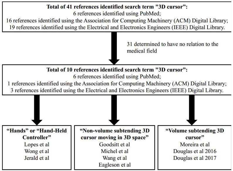
Moher D, Liberati A, Tetzlaff J, et al. (2009) Preferred reporting items for systematic reviews and meta-analyses: the PRISMA statement. PLoS medicine 6: e1000097. doi: 10.1371/journal.pmed.1000097
    [13] Lopes DS, de Figueiredo Parreira PD, Paulo SF, et al. (2017) On the utility of 3D hand cursors to explore medical volume datasets with a touchless interface. J biomed inform 72: 140–149. doi: 10.1016/j.jbi.2017.07.009
    [14] Wang W, Collinger JL, Degenhart AD, et al. (2013) An electrocorticographic brain interface in an individual with tetraplegia. PloS one 8: e55344. doi: 10.1371/journal.pone.0055344
    [15] Goodsitt MM, Chan HP, Hadjiiski L (2000) Stereomammography: Evaluation of depth perception using a virtual 3D cursor. Mel phys 27: 1305–1310.
    [16] Wong TZ, Lateiner JS, Mahon TG, et al. (1996) Stereoscopically guided characterization of three-dimensional dynamic MR images of the breast. Radiology 198: 288–291. doi: 10.1148/radiology.198.1.8539396
    [17] Park S, Kim S, Park J (2012) Select ahead: efficient object selection technique using the tendency of recent cursor movements. Asia-Pacific Computer and Human Interaction: 51–58.
    [18] Katzakis N, Kiyokawa K, Takemura H (2013) Plane-casting: 3D cursor control with a smartphone. Asia-Pacific Computer and Human Interaction: 199–200.
    [19] Hudson SE (1992) The interaction technique notebook: Adding shadows to a 3D cursor. ACM Transactions on Graphics (TOG) 11: 193–199. doi: 10.1145/130881.370599
    [20] Dorta T, Kinayoglu G, Hoffmann M (2015) Hyve-3D and rethinking the 3D cursor: unfolding a natural interaction model for remote and local co-design in VR. International Conference on Computer Graphics and Interactive Techniques: 43.
    [21] Biocca F, Tang A, Owen C, et al. (2006) Attention funnel: omnidirectional 3D cursor for mobile augmented reality platforms. Human Factors in Computing Systems: 1115–1122.
    [22] Jung T, Bauer P (2017) Constraint-based modeling technique for mid-air interaction. Symposium on Spatial User Interaction: 157–157.
    [23] Feng J, Wartell Z (2014) Riding the plane: bimanual, desktop 3D manipulation. User Interface Software and Technology: 93–94.
    [24] Brewer J, Anderson D (1976) Techniques for interactive three dimensional design. International Conference on Computer Graphics and Interactive Techniques: 13–30.
    [25] Venolia D (1993) Facile 3D direct manipulation. Human Factors in Computing Systems: 31–36.
    [26] Teather RJ, Stuerzlinger W (2012) A system for evaluating 3D pointing techniques. Virtual Reality Software and Technology: 209–210.
    [27] Elmqvist N (2005) BalloonProbe: Reducing occlusion in 3D using interactive space distortion. Virtual Reality Software and Technology: 134–137.
    [28] Brewer JA, Anderson DC (1977) Visual interaction with overhauser curves and surfaces. International Conference on Computer Graphics and Interactive Techniques 11: 132–137.
    [29] Jerald J, Yoganandan A (2011) iMedic: immersive medical environment for distributed interactive consultation. International Conference on Computer Graphics and Interactive Techniques: 99–99.
    [30] Menelas B-AJ (2013) Interactive analysis of cavity-flows in a virtual environment. Spring Conference on Computer Graphics: 31–37.
    [31] Serrar Z, Elmarzouqi N, Jarir Z, et al. (2014) Evaluation of Disambiguation Mechanisms of Object-Based Selection in Virtual Environment: Which Performances and Features to Support "Pick Out"? International Conference on Human-Computer Interaction: 29.
    [32] Ware C, Lowther K (1997) Selection using a one-eyed cursor in a fish tank VR environment. ACM Transactions on Computer-Human Interaction (TOCHI) 4: 309–322. doi: 10.1145/267135.267136
    [33] Biocca F, Tang A, Owen C, et al. (2006) The omnidirectional attention funnel: A dynamic 3D cursor for mobile augmented reality systems. Hawaii International Conference on System Sciences 1: 22c–22c.
    [34] Kadri A, Lécuyer A, Burkhardt J-M, et al. (2007) The Influence of Visual Appearance of User's Avatar on the Manipulation of Objects in Virtual Environments. IEEE Virtual Reality Conference: 291–292.
    [35] Young TS, Teather RJ, MacKenzie IS (2017) An arm-mounted inertial controller for 6DOF input: Design and evaluation. Symposium on 3D User Interfaces: 26–35.
    [36] Moreira DA, Hage C, Luque EF, et al. (2015) 3D markup of radiological images in ePAD, a web-based image annotation tool. Computer-Based Medical Sytems: 97–102.
    [37] Jáuregui DAG, Argelaguet F, Lecuyer A (2012) Design and evaluation of 3D cursors and motion parallax for the exploration of desktop virtual environments. Symposium on 3D User Interfaces: 69–76.
    [38] Kadri A, Lécuyer A, Burkhardt J-M (2007) The visual appearance of user's avatar can influence the manipulation of both real devices and virtual objects. Symposium on 3D User Interfaces: 11.
    [39] Wither J, Höllerer T (2005) Pictorial depth cues for outdoor augmented reality. International Symposium on Wearable Computers: 92–99.
    [40] Wither J, Höllerer T (2004) Evaluating techniques for interaction at a distance. International Symposium on Wearable Computers 1: 124–127.
    [41] Wu S-T, Abrantes M, Tost D, et al. (2003) Picking and snapping for 3d input devices. Brazilian Symposium on Computer Graphics and Image Processing: 140–147.
    [42] Schwartz AB, Tillery SH, Taylor DM (2003) Cortical control of natural arm movement. International IEEE/EMBS Conference on Neural Engineering: 99.
    [43] Adachi Y (1993) Touch and trace on the free-form surface of virtual object. IEEE Virtual Reality Conference: 162–168.
    [44] Stein T, Coquillart S (2000) The metric cursor. Pacific Conference on Computer Graphics and Applications: 381–386.
    [45] Michel C, Sibomana M, Bodart J-M, et al. (1995) Interactive delineation of brain sulci and their merging into functional PET images. Nuclear Science Symposium and Medical Imaging Conference 3: 1480–1484.
    [46] Ernst H, Petzold J, Larice R, et al. (1996) Mixing of computer graphics and high-quality stereographic video. IEEE transactions on consumer electronics 42: 795–799. doi: 10.1109/30.536187
    [47] Özacar K, Hincapié-Ramos JD, Takashima K, et al. (2016) 3D Selection Techniques for Mobile Augmented Reality Head-Mounted Displays. Interact Comput 29: 579–591.
    [48] Eagleson R, Wucherer P, Stefan P, et al. (2015) Collaborative table-top VR display for neurosurgical planning. IEEE Virtual Reality Conference: 169–170.
    [49] Ernst H, Petzold J, Larice R, et al. (1996) High-quality overlay of live stereo video on computer graphics. International Conference on Consumer Electronics: 404.
    [50] Taylor DM (2007) The importance of online error correction and feed-forward adjustment in brain-machine interfaces for restoration of movement. Toward Brain-computer Interfacing: 161.
    [51] Dang N-T (2007) A survey and classification of 3D pointing techniques. IEEE International Conference on Research, Innovation and Vision for the Future: 71–80.
    [52] Douglas DB, Wilke CA, Gibson D, et al. (2017) Virtual reality and augmented reality: Advances in surgery. Biol 2: 1–8.
    [53] Hinckley K, Pausch R, Goble JC, et al. (1994) Passive real-world interface props for neurosurgical visualization. Human Factors in Computing Systems: 452–458.
    [54] David Douglas MDCW, M.S.; David Gibson, M.S.; Emanuel Petricoin, Ph.D.; Lance Liotta, Ph.D.; Demetri Venets, B.S.; Buddy Beck, M.B.A.; Robert Douglas, Ph.D. (2018) Depth-3-Dimensional (D3D) Augmented Reality Viewing of a Lung Cancer Imaged with PET: Proof of Concept. SNMMI Mid-Winter Meeting 2018. Orlando, FL.
  • Reader Comments
  • © 2018 the Author(s), licensee AIMS Press. This is an open access article distributed under the terms of the Creative Commons Attribution License (http://creativecommons.org/licenses/by/4.0)
通讯作者: 陈斌, bchen63@163.com
  • 1. 

    沈阳化工大学材料科学与工程学院 沈阳 110142

  1. 本站搜索
  2. 百度学术搜索
  3. 万方数据库搜索
  4. CNKI搜索

Metrics

Article views(5707) PDF downloads(995) Cited by(2)

/

DownLoad:  Full-Size Img  PowerPoint
Return
Return

Catalog