Geoinformatic analysis of vegetation and climate change on intertidal sedimentary landforms in southeastern Australian estuaries from 1975–2015

Ali K. M. Al-Nasrawi; Sarah M. Hamylton; Brian G. Jones; Ameen A. Kadhim; Ali K. M. Al-Nasrawi; Sarah M. Hamylton; Brian G. Jones; Ameen A. Kadhim

doi:10.3934/geosci.2018.1.36

AIMS Geosciences

2018, Volume 4, Issue 1: 36-65. doi: 10.3934/geosci.2018.1.36

Previous Article Next Article

Research article

Geoinformatic analysis of vegetation and climate change on intertidal sedimentary landforms in southeastern Australian estuaries from 1975–2015

1.
GeoQuEST Research Centre, School of Earth and Environmental Sciences, University of Wollongong, NSW 2522, Australia
2.
Department of Geography, Environment and Spatial Sciences, Michigan State University, Michigan, USA

Received: 18 December 2017 Accepted: 19 March 2018 Published: 23 March 2018

Vegetation canopies represent the main ecosystems on intertidal landforms and they clearly respond to changes in coastal environments. Climate change, including temperature, precipitation and sea level rise, are affecting the health and distribution of coastal vegetation, as well as the runoff and sedimentation rates that can impact coastal areas. This study has used the normalized difference vegetation index (NDVI) to investigate vegetation canopy dynamics on three different coastal sites in southeastern Australia over the past 47 years (1975–2015). NDVIs temporal-datasets have been built from satellite images derived from Landsat 1–8. These were then regressed to the climatic and geomorphic variables. Results show clear increases in NDVI at Towamba and Wandandian Estuaries, but a decline at Comerong Island (southeastern Australia). The sedimentation rate has the most significant positive impact on NDVI since it has the potential to provide additional space for vegetation. Temperature and sea level rise have positive effects, except on Comerong Island, but rainfall has no significant effect on the NDVI at any site. Different NDVI trends have been recorded at these three coastal sites reflecting different correlations between the vegetation, climatic and geomorphic (as independent) variables. The geomorphological characteristics of the highly-dynamic intertidal estuarine landforms, which are subject to active erosion and deposition processes, have the largest impact on vegetation cover and, hence, on NDVI. Assessing the vegetation canopy using NDVI as an evaluation tool has provided temporal-dynamic datasets that can be correlated to the main individual environmental controls. Such knowledge will allow resource managers to make more informed decisions for sustainable conservation plans following the evaluation the potential consequences of any environmental changes.
- ecosystems,
- climate change,
- vegetation response,
- NDVI,
- GIS analyses,
- remote sensing,
- satellite imagery
Citation: Ali K. M. Al-Nasrawi, Sarah M. Hamylton, Brian G. Jones, Ameen A. Kadhim. Geoinformatic analysis of vegetation and climate change on intertidal sedimentary landforms in southeastern Australian estuaries from 1975–2015[J]. AIMS Geosciences, 2018, 4(1): 36-65. doi: 10.3934/geosci.2018.1.36

Related Papers:

Abstract

Vegetation canopies represent the main ecosystems on intertidal landforms and they clearly respond to changes in coastal environments. Climate change, including temperature, precipitation and sea level rise, are affecting the health and distribution of coastal vegetation, as well as the runoff and sedimentation rates that can impact coastal areas. This study has used the normalized difference vegetation index (NDVI) to investigate vegetation canopy dynamics on three different coastal sites in southeastern Australia over the past 47 years (1975–2015). NDVIs temporal-datasets have been built from satellite images derived from Landsat 1–8. These were then regressed to the climatic and geomorphic variables. Results show clear increases in NDVI at Towamba and Wandandian Estuaries, but a decline at Comerong Island (southeastern Australia). The sedimentation rate has the most significant positive impact on NDVI since it has the potential to provide additional space for vegetation. Temperature and sea level rise have positive effects, except on Comerong Island, but rainfall has no significant effect on the NDVI at any site. Different NDVI trends have been recorded at these three coastal sites reflecting different correlations between the vegetation, climatic and geomorphic (as independent) variables. The geomorphological characteristics of the highly-dynamic intertidal estuarine landforms, which are subject to active erosion and deposition processes, have the largest impact on vegetation cover and, hence, on NDVI. Assessing the vegetation canopy using NDVI as an evaluation tool has provided temporal-dynamic datasets that can be correlated to the main individual environmental controls. Such knowledge will allow resource managers to make more informed decisions for sustainable conservation plans following the evaluation the potential consequences of any environmental changes.

References

[1]	Costanza R, (1999) Ecological sustainability, indicators, and climate change, In: IPCC Expert Meeting on Development, Equity and Sustainability, Colombo, Sri Lanka, Citeseer.
[2]	Pittock AB (2003) Climate change: An Australian guide to the science and potential impacts. Aust Greenhouse Off Canberra.
[3]	Zinnert J, Shiflett S, Vick J, et al. (2011) Woody vegetative cover dynamics in response to recent climate change on an Atlantic coast barrier island: A remote sensing approach. Geocarto Int 26: 595–612. doi: 10.1080/10106049.2011.621031
[4]	IPCC, (2014) Climate Change 2014: Synthesis Report. In: Core Writing Team, R.K. Pachauri and L.A. Meyer, Eds., Contribution of Working Groups I, II and III to the Fifth Assessment Report of the Intergovernmental Panel on Climate Change, Geneva, Switzerland, 151.
[5]	Goward SN, Prince SD (1995) Transient effects of climate on vegetation dynamics: Satellite observations. J Biogeography 22: 549–564. doi: 10.2307/2845953
[6]	Donohue RJ, Mcvicar TR, Roderick ML (2010) Climate‐related trends in Australian vegetation cover as inferred from satellite observations, 1981–2006. Global Change Biology 15: 1025–1039.
[7]	Woodroffe CD (1990) The impact of sea-level rise on mangrove shorelines. Prog Phys Geogr 14: 483–520. doi: 10.1177/030913339001400404
[8]	Michener WK, Blood ER, Bildstein KL, et al. (1997) Climate change, hurricanes and tropical storms, and rising sea level in coastal wetlands. Ecol Appl 7: 770–801. doi: 10.1890/1051-0761(1997)007[0770:CCHATS]2.0.CO;2
[9]	Scavia D, Field JC, Boesch DF, et al. (2002) Climate change impacts on US coastal and marine ecosystems. Estuaries 25: 149–164. doi: 10.1007/BF02691304
[10]	Day JW, Christian RR, Boesch DM, et al. (2008) Consequences of climate change on the ecogeomorphology of coastal wetlands. Estuaries Coasts 31: 477–491. doi: 10.1007/s12237-008-9047-6
[11]	Meyssignac B, Cazenave A (2012) Sea level: A review of present-day and recent-past changes and variability. J Geodyn 58: 96–109. doi: 10.1016/j.jog.2012.03.005
[12]	Mitsch WJ, Gosselink JG (2015) Wetlands 5th edition, Wiley, New Jersey, 744pp.
[13]	NCCMA (1998) The role of wetlands Fact Sheet Project 1559. North Central Catchment Management Authority, Huntly, Victoria, 2pp.
[14]	DSE, (2007) Index of Wetland Condition (Review of wetland assessment methods), Department of Sustainability and Environment: S.A. Melbournethe, Victorian Government.
[15]	Al-Nasrawi AKM, Jones BG, Alyazichi YM, et al. (2015) Modelling the future eco-geomorphological change scenarios of coastal ecosystems in southeastern Australia for sustainability assessment using GIS, In: ACSUS 2015 Proceedings: The Second Asian Conference on the Social Sciences and Sustainability, Japan, 0196.
[16]	Al-Nasrawi AKM, Jones BG, Alyazichi YM, et al. (2016) Civil-GIS incorporated approach for water resource management in a developed catchment for urban-geomorphic sustainability: Tallowa Dam, southeastern Australia. Int Soil Water Conserv Res 4: 304–313. doi: 10.1016/j.iswcr.2016.11.001
[17]	Al-Nasrawi AKW, Jones BG, Hamylton SM (2016) GIS-based modelling of vulnerability of coastal wetland ecosystems to environmental changes: Comerong Island, southeastern Australia. J Coastal Res 2016: 33–37.
[18]	Hughes L (2003) Climate change and Australia: Trends, projections and impacts. Aust Ecol 28: 423–443. doi: 10.1046/j.1442-9993.2003.01300.x
[19]	Nicholls RJ (2004) Coastal flooding and wetland loss in the 21st century: Changes under the SRES climate and socio-economic scenarios. Global Environ Change 14: 69–86. doi: 10.1016/j.gloenvcha.2003.10.007
[20]	Blay J (1944) On Track: Searching out the Bundian Way, Eden local history reference collection. Sydney: NewSouth Publishing.
[21]	Wright LD (1970) The influence of sediment availability on patterns of beach ridge development in the vicinity of the Shoalhaven river delta, N.S.W. Aust Geogr 11: 336–348. doi: 10.1080/00049187008702570
[22]	Hopley CA (2013) Autocyclic, allocyclic and anthropogenic impacts on Holocene delta evolution and future management implications: Macquarie Rivulet and Mullet/Hooka Creek, Lake Illawarra, New South Wales. PhD thesis, University of Wollongong, Australia, 338.
[23]	OEH (2013) Assessing estuary ecosystem health: Sampling, data analysis and reporting protocols: NSW Natural Resources Monitoring, Evaluation and Reporting Program. State of NSW and Office of Environment and Heritage, 3–38.
[24]	Kirkpatrick S, (2012) The Economic Value of Natural and Built Coastal Assets: Part 2: Built Coastal Assets, In: Australian Climate Change Adaptation Research Network for Settlements and Infrastructure, National Climate Change Adaptation Research Facility.
[25]	Pendleton LH (2010) The economic and market value of coasts and estuaries: What's at stake? Economic 175.
[26]	Roy PS, Williams RJ, Jones AR, et al. (2001) Structure and function of south-east Australian estuaries. Estuarine Coastal Shelf Sci 53: 351–384. doi: 10.1006/ecss.2001.0796
[27]	Al-Nasrawi AKM, Hamylton SM, Jones BG (2018) Spatio-temporal assessment of anthropogenic and climate stressors on estuaries using a GIS-modelling approach for sustainability; Towamba estuary, southeastern Australia. Environ Monit Assess J.
[28]	Al-Nasrawi A, Hopley C, Hamylton S, et al. (2017) A Spatio-Temporal Assessment of Landcover and Coastal Changes at Wandandian Delta System, Southeastern Australia. J Mar Sci Eng 5: 55. doi: 10.3390/jmse5040055
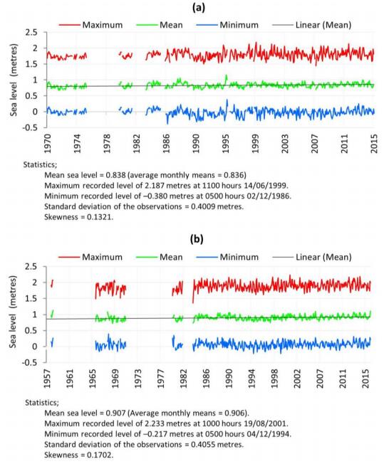
[29]	Bureau of Meterology. NSW Weather, 2017. Available from: http://www.bom.gov.au.
[30]	Dean LF, Deckker PD (2013) Recent benthic foraminifera from Twofold Bay, Eden NSW: Community structure, biotopes and distribution controls. J Geol Soc Aust 60: 475–496.
[31]	DPI/OW. NSW Office of Water-NEW Government-Department of Primary Industries, 2017. Available from: http://www.water.nsw.gov.au/.
[32]	Hudson JP, (1991) Late Quaternary Evolution of Twofold Bay, Southern New South Wales, In: Department of Geography, University of Sydney: Unpublished.
[33]	Jones CAHBG (2006) Holocene stratigraphic and morphological evolution of the Wandandian Creek delta, St Georges Basin, New South Wales. J Geol Soc Aust 53: 991–1000.
[34]	Kingsford RT (1990) The effects of human activities on shorebirds, seabirds and waterbirds of Comerong Island, at the mouth of the Shoalhaven River. Wetlands 9: 7–12.
[35]	Christian AT, Hill SM (2002) Regolith-landform mapping of the Shoalhaven River Delta and hinterland, NSW: Towards a model for landscape change and management. Regolith Landscapes East Aust 8–13.
[36]	Umitsu M, Buman M, Kawase K, et al. (2001) Holocene palaeoecology and formation of the Shoalhaven River deltaic-estuarine plains, southeast Australia. Holocene 11: 407–418. doi: 10.1191/095968301678302841
[37]	Thompson CM, (2012) Recent Dynamic Channel Adjustments of Berrys Canal Shoalhaven Region, New South Wales Approach, In: B.Env.Sc. thesis, University of Wollongong.
[38]	DEE. Coasts and oceans: Ecosystem conditions, 2006. Available from: https://www.environment.gov.au/node/21960.
[39]	Bureau of Meteorology. Climate classification of Australia, 2017. Available from: http://www.bom.gov.au/climate/.
[40]	Fensham RJ, Fairfax RJ, Archer SR (2005) Rainfall, land use and woody vegetation cover change in semi‐arid Australian savanna. J Ecol 93: 596–606. doi: 10.1111/j.1365-2745.2005.00998.x
[41]	Semeniuk C, Semeniuk V (2013) The response of basin wetlands to climate changes: A review of case studies from the Swan Coastal Plain, south-western Australia. Hydrobiologia 708: 45–67. doi: 10.1007/s10750-012-1161-6
[42]	KNMI-Climate_Explorer. Select a monthly time series, 2018. Available from: https://climexp.knmi.nl/selectstation.cgi?id=someone@somewhere.
[43]	Raynolds M, Magnússon B, Metúsalemsson S, et al. (2015) Warming, sheep and volcanoes: Land cover changes in Iceland evident in satellite NDVI trends. Remote Sens 7: 9492–9506. doi: 10.3390/rs70809492
[44]	Weier J, Herring D (2000) Measuring Vegetation (NDVI & EVI). Available from: http://earthobservatory.nasa.gov/Features/MeasuringVegetation/.
[45]	Pettorelli N, Vik JO, Mysterud A, et al. (2005) Using the satellite-derived NDVI to assess ecological responses to environmental change. Trends Ecol Evol 20: 503–510. doi: 10.1016/j.tree.2005.05.011
[46]	Church JA (2013) Projections of sea level rise IPCC AR5. Clim Change 2013: 1137–1216.
[47]	Gedan KB, Kirwan ML, Wolanski E, et al. (2011) The present and future role of coastal wetland vegetation in protecting shorelines: Answering recent challenges to the paradigm. Clim Change 106: 7–29. doi: 10.1007/s10584-010-0003-7
[48]	Costanza R, Pérez-Maqueo O, Martinez ML, et al. (2008) The value of coastal wetlands for hurricane protection. Ambio 37: 241–248. doi: 10.1579/0044-7447(2008)37[241:TVOCWF]2.0.CO;2
[49]	Lee SY, Rjk D, Young RA, et al. (2006) Impact of urbanization on coastal wetland structure and function. Aust Ecol 31: 149–163. doi: 10.1111/j.1442-9993.2006.01581.x
[50]	Department of Environment, (2010) Riverine Ecosystems, Southern river Region, In: State of the Catchments, New South Wales Government.
[51]	Thom BG (1967) Mangrove ecology and deltaic geomorphology: Tabasco, Mexico. J Ecol 55: 301–343. doi: 10.2307/2257879
[52]	Deconto RM, Pollard D (2016) Contribution of Antarctica to past and future sea-level rise. Nature 531: 591–597. doi: 10.1038/nature17145
[53]	Neumann B, Vafeidis AT, Zimmermann J, et al. (2015) Future Coastal Population Growth and Exposure to Sea-Level Rise and Coastal Flooding-A Global Assessment. PloS One 10: e0118571. doi: 10.1371/journal.pone.0118571
[54]	Pachauri RK, Team CW, Meyer LA (2014) Climate Change 2014: Synthesis Report. Contribution of Working Groups I, II and III to the Fifth Assessment Report of the Intergovernmental Panel on Climate Change. J Romance Stud 4: 85–88.
[55]	Bureau of Meterology-NSW. Tide Gauge Metadata and Observed Monthly Sea Levels and Statistics, 2017. Available from: http://www.bom.gov.au/oceanography/projects/ntc/monthly/.
[56]	USGS. EarthExplorer, 2017. Available from: http://earthexplorer.usgs.gov/.
[57]	USGS-Landsat. Landsat Collections, 2017. Available from: http://landsat.usgs.gov//landsatcollections.php.
[58]	Nguyrobertson AL, Gitelson AA (2015) Algorithms for estimating green leaf area index in C3 and C4 crops for MODIS, Landsat TM/ETM+, MERIS, Sentinel MSI/OLCI, and Venµs sensors. Remote Sens Lett 6: 360–369. doi: 10.1080/2150704X.2015.1034888
[59]	Peng Y, Nguy-Robertson A, Arkebauer T, et al. (2017) Assessment of canopy chlorophyll content retrieval in maize and soybean: Implications of hysteresis on the development of generic algorithms. Remote Sens 9: 226. doi: 10.3390/rs9030226
[60]	Feng T, Fensholt R, Verbesselt J, et al (2015) Evaluating temporal consistency of long-term global NDVI datasets for trend analysis. Remote Sens Environ 163: 326–340. doi: 10.1016/j.rse.2015.03.031
[61]	Curtis E (2016) The use of Landsat derived vegetation metrics in Generalised Linear Mixed Modelling of River Red Gum (Eucalyptus camaldulensis) canopy condition dynamics in Murray Valley National Park, NSW, between 2008 and 2016. University of Wollongong, Wollongong, Australia, 148.
[62]	Cordeiro JPC, Câmara G, Moura UF, et al. (2005) Algebraic Formalism over Maps. Geoinfo 2008: 49–65.
[63]	Esri. A quick tour of using Map Algebra-ArcGIS Help \| ArcGIS Desktop, 2017. Available from: http://desktop.arcgis.com/en/arcmap/latest/extensions/spatial-analyst/map-algebra/a-quick-tour-of-using-map-algebra.htm.
[64]	Lambin EF, Strahlers AH (1994) Change-vector analysis in multitemporal space: A tool to detect and categorize land-cover change processes using high temporal-resolution satellite data. Remote Sens Environ 48: 231–244. doi: 10.1016/0034-4257(94)90144-9
[65]	Zanchetta A, Bitelli G (2017) A combined change detection procedure to study desertification using opensource tools. Open Geospatial Data Software Stand 2: 10. doi: 10.1186/s40965-017-0023-6
[66]	Li J, Xu B, Yang X, et al. (2017) Historical grassland desertification changes in the Horqin Sandy Land, Northern China (1985–2013). Sci Rep 7: 3009. doi: 10.1038/s41598-017-03267-x
[67]	Al-Nasrawi A, Jones B, Hamylton S, (2015) Modelling changes of coastal wetlands responding to disturbance regimes (Eastern Australia), In: Australian Mangrove and Saltmarsh Network Conference : Working with Mangrove and Saltmarsh for Sustainable Outcomes, Wollongong, Australia: Australian Mangrove and Saltmarsh Network, 33.
[68]	Al-Nasrawi AKM (2017) Surface Elevation Dynamics Assessment Using Digital Elevation Models, Light Detection and Ranging, GPS and Geospatial Information Science Analysis: Ecosystem Modelling Approach. Int J Environ 131: 918–923.
[69]	Carvalho RC, Woodroffe C, (2013) Shoalhaven river mouth: A retrospective analysis of breaching using aerial photography, landsatimagery and LiDAR, In: In Proceedings of the 34th Asian Conference on Remote Sensing 2013, Indonesian Remote Sensing Society, Indonesia, 1–7.
[70]	Hopley CA (2004) The Holocene and beyond: Evolution of Wandandian Creek delta, St Georges Basin, New South Wales. BSc(Hons) thesis, University of Wollongong, Australia.
[71]	WRC, Wetland Mapping: Exercises-Create the NDVI Layer ArcMap 10. Water Resources Center (WRC), University of Minnesota [Online], 2012. Available from: https://www.wrc.umn.edu/sites/wrc.umn.edu/files/create_the_ndvi.pdf.

Reader Comments

Your name:*

Email:*
© 2018 the Author(s), licensee AIMS Press. This is an open access article distributed under the terms of the Creative Commons Attribution License (http://creativecommons.org/licenses/by/4.0)