Phytochemical comparison with quantitative analysis between two flower phenotypes of <em>Mentha aquatica</em> L.: pink-violet and white

Alessandro Venditti; Claudio Frezza; Diana Celona; Fabio Sciubba; Sebastiano Foddai; Maurizio Delfini; Mauro Serafini; Armandodoriano Bianco

doi:10.3934/molsci.2017.3.288

AIMS Molecular Science, 2017, 4(3): 288-300. doi: 10.3934/molsci.2017.3.288. Research article

Export file:

Format

RIS(for EndNote,Reference Manager,ProCite)
BibTex
Text

Content

Citation Only
Citation and Abstract

Phytochemical comparison with quantitative analysis between two flower phenotypes of Mentha aquatica L.: pink-violet and white

Alessandro Venditti, Claudio Frezza, Diana Celona, Fabio Sciubba, Sebastiano Foddai, Maurizio Delfini, Mauro Serafini, Armandodoriano Bianco

1 Dipartimento di Chimica, Sapienza Università di Roma, P.le Aldo Moro, 5-00185 Roma, Italy
2 Dipartimento Biologia Ambientale, Sapienza Università di Roma, P.le Aldo Moro, 5-00185 Roma, Italy

Received: , Accepted: , Published:

Abstract Full Text(HTML) Figure/Table Supplementary Related pages

In this work, the first phytochemical comparison performed on the polar fractions of two different phenotypes of Mentha aquatica L. having pink-violet and white flowers, is reported. This comparison was conducted through both a classical phytochemical analysis and a metabolomic one by means of spectroscopic and spectrometric approaches. Twenty-seven compounds were identified in both phenotypes. Most of them were evidenced in both. Anyway, all these compounds possess chemotaxonomic, pharmacological and nutritional value. In particular, one compound represents a new phytochemical for the species and two other compounds are new phytochemicals for the genus, instead. The results obtained allowed us to ascertain, from a phytochemical standpoint, that also this species can be used as possible medicinal plant like all the other species of this genus and as a source of important nutritional factors due to the presence of compounds with high nutritional properties.

Figure/Table

Supplementary

Article Metrics

Keywords: Mentha aquatica L.; pink-violet flowers; white flowers; phytochemical analysis; phytochemical comparison; quantitative analysis

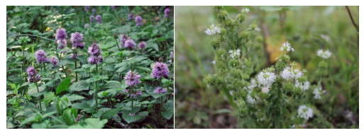
Citation: Alessandro Venditti, Claudio Frezza, Diana Celona, Fabio Sciubba, Sebastiano Foddai, Maurizio Delfini, Mauro Serafini, Armandodoriano Bianco. Phytochemical comparison with quantitative analysis between two flower phenotypes of Mentha aquatica L.: pink-violet and white. AIMS Molecular Science, 2017, 4(3): 288-300. doi: 10.3934/molsci.2017.3.288

References:

1. Pignatti S (1982) Flora d'Italia, Eds., Bologna: Edagricole, 496.
2. Conti F, Abbate G, Alessandrini A, et al. (2005) An annotated Checklist of the Italian vascular flora, Rome: Palombi.
3. Lanzara P (1997) Piante medicinali, Torriana: Orsa Maggiore Editore .
4. Sylianco CYL, Blanco F R, Lim CM (1987) Mutagenicity, clastogenicity and antimutagenicity of medicinal plant tablets produced by the NSTA pilot plant IV, Yerba buena tablets. Philipp J Sci 115: 299-305.
5. Tyler VE (1993) The honest herbal, 3Eds, Binghamton: Pharmaceutical Products Press.
6. Bisset NG (1994) Herbal Drugs, Stuttgart: Medpharm Scientific Publishers.
7. Hendriks H (1998) Pharmaceutical aspects of some Mentha herbs and their essential oils. Perfum Flavor 23: 15-23.
8. Başer KHC, Kürkcüoglu M, Tarimicilar G, et al. (1999) Essential oils of Mentha species from northern Turkey. J Essent Oil Res 11: 579-588.
9. El-Gohary AE, El-Sherbeny SE, Ghazal GMEM, et al. (2014) Evaluation of essential oil and monoterpenes of peppermint (Mentha piperita L.) under humic acid with foliar nutrition. J Mater Environ Sci 5: 1885-1890.
10. Guarrera PM, Savo V (2016) Wild food plants used in traditional vegetable mixtures in Italy. J Ethnopharmacol 185: 202-234.
11. Senatore F, D'Alessio A, Formisano C, et al. (2005) Chemical composition and antibacterial activity of the essential oil of a 1,8-Cineole chemotype of Mentha aquatica L. growing Wild in Turkey. J Essent Oil Bear Plants 8: 148-153.
12. Esmaeili A, Rustaiyan A, Masoudi S, et al. (2006) Composition of the Essential Oils of Mentha aquatica L. and Nepeta meyeri Benth. from Iran. J Essent Oil Res 18: 263-265.
13. Voirin B, Bayet C, Faurec O, et al. (1999) Free flavonoid aglycones as markers of parentage in Mentha aquatica, M. citrata, M. spicata and M. piperita. Phytochem 50: 1189-1193.
14. Olsen HT, Stafford GI, Van Staden J, et al. (2008) Isolation of the MAO-inhibitor naringenin from Mentha aquatica L. J Ethnopharmacol 117: 500-502.
15. Venditti A, Frezza C, Riccardelli M, et al. (2016) Unusual molecular pattern in Ajugoideae subfamily: the case of Ajuga genevensis L. from Dolomites. Nat Prod Res 30: 1098-1102.
16. Sciubba F, Capuani G, Di Cocco ME, et al. (2014) Nuclear magnetic resonance analysis of water soluble metabolites allows the geographic discrimination of pistachios (Pistacia vera). Food Res Int 62: 66-73.
17. Rothman DL., Petroff OAC, Behar KL, et al. (1993) Localized ¹H NMR measurements of y-aminobutyric acid in human brain in vivo. Proc Nat Acad Sci USA 90: 5662-5666.
18. Pauli GF, Poetsch F, Nahrstedt A (1988) Structure assignment of natural quinic acid derivatives using proton nuclear magnetic resonance techniques. Phytochem Analysis 9: 177-185.
19. Jadrijevi-Mladar Takaĉ M, Vikiĉ Topiĉ D (2004) FT-IR and NMR spectroscopic studies of salicylic acid derivatives. II. Comparison of 2-hydroxy- and 2,4- and 2,5-dihydroxy derivatives. Acta Pharm 54: 177-191.
20. Sciubba F, Di Cocco ME, Gianferri R, et al. (2014) Metabolic profile of different Italian cultivars of hazelnut (Corylus avellana) by nuclear magnetic resonance spectroscopy. Nat Prod Res 28: 1075-1081.
21. Aguirre C, Delporte C, Backhouse N, et al. (2006) Topical anti-inflammatory activity of 2a-hydroxy pentacyclic triterpene acids from the leaves of Ugni molinae. Bioorg Med Chem Lett 14: 5673-5677.
22. Shekarchi M, Hajimehdipoor H, Saeidnia S, et al. (2012) Comparative study of rosmarinic acid content in some plants of Labiatae family. Pharmacogn Mag 8: 37-41.
23. Bai N, He K, Roller M, et al. (2010) Flavonoids and phenolic compounds from Rosmarinus officinalis. J Agric Food Chem 58: 5363-5367.
24. Pedersen JA (2000) Distribution and taxonomic implications of some phenolics in the family Lamiaceae determined by ESR spectroscopy. Biochem Syst Ecol 28: 229-253.
25. Karasawa D, Shimizu S (1980) Triterpene acids in callus tissues from Mentha arvensis var. piperascens Mal. Agr Biol Chem 44: 1203-1205.
26. Suga T, Hirata T, Yamamoto Y (1980) Lipid constituents of callus tissues of Mentha spicata. Agr Biol Chem 44: 1817-1820.
27. Kokdil G, Topcu G, Goren A C, et al. (2002) Steroids and terpenoids from Ajuga relicta. Zeitschrift für Naturforschung B 57: 957-960.
28. Aladedunye FA, Okorie DA, Ighodaro OM (2008) Anti-inflammatory and antioxidant activities and constituents of Platostoma africanum P. Beauv. Nat Prod Res 22: 1067-1073.
29. Zielińska S, Matkowski A (2014) Phytochemistry and bioactivity of aromatic and medicinal plants from the genus Agastache (Lamiaceae). Phytochem Rev 13: 391-416.
30. Al-Dhabi NA., Arasu MV, Park CH, et al. (2014) Recent studies on rosmarinic acid and its biological and pharmacological activities. Exclie J 13: 1192-1195.
31. Liu J (1995) Pharmacology of oleanolic acid and ursolic acid. J Ethnopharmacol 49: 57-68.
32. Ahn K, Hahm M S, Park E J, et al. (1998) Corosolic acid isolated from the fruit of Crataegus pinnatifida var. psilosa is a protein kinase C inhibitor as well as a cytotoxic agent. Planta Med 64: 468-470.
33. Bunbupha S, Prachaney P, Kukongviriyapan U, et al. (2015) Asiatic acid alleviates cardiovascular remodelling in rats with L-NAME-induced hypertension. Clin Exp Pharmacol P 42: 1189-1197.
34. Zhou J, Chan L, Zhou S (2012) Trigonelline: a plant alkaloid with therapeutic potential for diabetes and central nervous system disease. Curr Med Chem 19: 3523-3531.
35. Stoll AL , Sachs GS, Cohen BM, et al. (1996) Choline in the treatment of rapid-cycling bipolar disorder: clinical and neurochemical findings in lithium-treated patients. Biol Psychiatry 40: 382-388.
36. Chan KC, So KF, Wu EX (2009) Proton magnetic resonance spectroscopy revealed choline reduction in the visual cortex in an experimental model of chronic glaucoma. Expe Eye Res 88: 65-70.
37. Zeisel SH, da Costa KA (2009) Choline: an essential nutrient for public health. Nutr Rev 67: 615-623.
38. Van Beek AH, Claassen JA (2010) The cerebrovascular role of the cholinergic neural system in Alzheimer's disease. Behav Brain Res 221: 537-542.
39. Nagoba BS, Selkar SP, Wadher BJ, et al. (2013) Acetic acid treatment of pseudomonal wound infections - a review. J infect public health 6: 410-415.
40. Matsuno T (1992) Isolation and characterization of the tumoricidal substances from Brazilian propolis. Honeybee Sci 13: 49-54.
41. Olthof M R, Hollman PC, Katan MB (2001) Chlorogenic acid and caffeic acid are absorbed in humans. J Nutr 131: 66-71.
42. Bhat RM, Vidya K, Kamath G, et al. (2001) Topical formic acid puncture technique for the treatment of common warts. Int J Dermatol 40: 415-419.
43. Chapouthier G, Venault P (2001) A pharmacological link between epilepsy and anxiety?. Trends Pharmacol Sci 22: 491-493.
44. Foster AC, Kemp JA (2006) Glutamate- and GABA-based CNS therapeutics. Curr Opin Pharmacol 6: 7-17.
45. Madan RK, Levitt J (2014) A review of toxicity from topical salicylic acid preparations. J Am Acad Dermatol 70: 788-792.
46. Catapano A L, Reiner Z, De Backer G, et al. (2011) ESC/EAS Guidelines for the management of dyslipidaemias: the Task Force for the management of dyslipidaemias of the European Society of Cardiology (ESC) and the European Atherosclerosis Society (EAS). Atherosclerosis 217:S1-44.
47. Hietala J, Vuori A, Johnsson P, et al. (2016) Formic Acid, In: Ullmann's Encyclopedia of Industrial Chemistry. Wiley, 1-22.
48. Zeikus JG, Jain MK, Elankovan P (1999) Biotechnology of succinic acid production and markets for derived industrial products. Appl Microbiol Biot 51: 545.

show all references

This article has been cited by:

1. Claudio Frezza, Alessandro Venditti, Mauro Serafini, Armandodoriano Bianco, , , 2019, 125, 10.1016/B978-0-444-64185-4.00004-6
2. Majid Mohammadhosseini, Alessandro Venditti, Abolfazl Akbarzadeh, The genus Perovskia Kar.: ethnobotany, chemotaxonomy and phytochemistry: a review, Toxin Reviews, 2019, 1, 10.1080/15569543.2019.1691013

Reader Comments

your name: * your email: *

Copyright Info: 2017, Alessandro Venditti, et al., licensee AIMS Press. This is an open access article distributed under the terms of the Creative Commons Attribution Licese (http://creativecommons.org/licenses/by/4.0)

Download full text in PDF

Associated material

Metrics