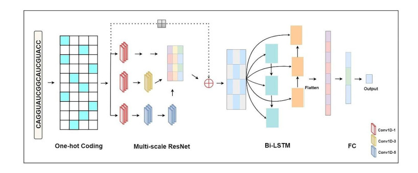
Phasic small interfering RNAs are plant secondary small interference RNAs that typically generated by the convergence of miRNAs and polyadenylated mRNAs. A growing number of studies have shown that miRNA-initiated phasiRNA plays crucial roles in regulating plant growth and stress responses. Experimental verification of miRNA-initiated phasiRNA loci may take considerable time, energy and labor. Therefore, computational methods capable of processing high throughput data have been proposed one by one. In this work, we proposed a predictor (DIGITAL) for identifying miRNA-initiated phasiRNAs in plant, which combined a multi-scale residual network with a bi-directional long-short term memory network. The negative dataset was constructed based on positive data, through replacing 60% of nucleotides randomly in each positive sample. Our predictor achieved the accuracy of 98.48% and 94.02% respectively on two independent test datasets with different sequence length. These independent testing results indicate the effectiveness of our model. Furthermore, DIGITAL is of robustness and generalization ability, and thus can be easily extended and applied for miRNA target recognition of other species. We provide the source code of DIGITAL, which is freely available at https://github.com/yuanyuanbu/DIGITAL.
Citation: Yuanyuan Bu, Jia Zheng, Cangzhi Jia. An efficient deep learning based predictor for identifying miRNA-triggered phasiRNA loci in plant[J]. Mathematical Biosciences and Engineering, 2023, 20(4): 6853-6865. doi: 10.3934/mbe.2023295
Phasic small interfering RNAs are plant secondary small interference RNAs that typically generated by the convergence of miRNAs and polyadenylated mRNAs. A growing number of studies have shown that miRNA-initiated phasiRNA plays crucial roles in regulating plant growth and stress responses. Experimental verification of miRNA-initiated phasiRNA loci may take considerable time, energy and labor. Therefore, computational methods capable of processing high throughput data have been proposed one by one. In this work, we proposed a predictor (DIGITAL) for identifying miRNA-initiated phasiRNAs in plant, which combined a multi-scale residual network with a bi-directional long-short term memory network. The negative dataset was constructed based on positive data, through replacing 60% of nucleotides randomly in each positive sample. Our predictor achieved the accuracy of 98.48% and 94.02% respectively on two independent test datasets with different sequence length. These independent testing results indicate the effectiveness of our model. Furthermore, DIGITAL is of robustness and generalization ability, and thus can be easily extended and applied for miRNA target recognition of other species. We provide the source code of DIGITAL, which is freely available at https://github.com/yuanyuanbu/DIGITAL.

| [1] |
B. He, J. Huang, H. Chen, PVsiRNAPred: Prediction of plant exclusive virus-derived small interfering RNAs by deep convolutional neural network, J Bioinform. Comput. Biol., 17 (2019), 1950039. https://doi.org/10.1142/S0219720019500392 doi: 10.1142/S0219720019500392

|
| [2] |
D. Baulcombe, RNA silencing in plants, Nature, 431 (2004), 356-363. https://doi.org/10.1038/nature02874 doi: 10.1038/nature02874
|
| [3] |
E. J. Chapman, J. C. Carrington, Specialization and evolution of endogenous small RNA pathways, Nat. Rev. Genet., 8 (2007), 884-896. https://doi.org/10.1038/nrg2179 doi: 10.1038/nrg2179
|
| [4] |
M. Niu, Y. Lin, Q. Zou, sgRNACNN: Identifying sgRNA on-target activity in four crops using ensembles of convolutional neural networks, Plant. Mol. Biol., 105 (2021), 483-495. https://doi.org/10.1007/s11103-020-01102-y doi: 10.1007/s11103-020-01102-y
|
| [5] |
S. M. Hammond, E. Bernstein, D. Beach, G. J. Hannon, An RNA-directed nuclease mediates post-transcriptional gene silencing in Drosophila cells, Nature, 404 (2000), 293-296. https://doi.org/10.1038/35005107 doi: 10.1038/35005107
|
| [6] |
S.-W. Ding, R. Lu, Virus-derived siRNAs and piRNAs in immunity and pathogenesis, Curr. Opin. Virol., 1 (2011), 533-544. https://doi.org/10.1016/j.coviro.2011.10.028 doi: 10.1016/j.coviro.2011.10.028
|
| [7] |
X. Chen, Small RNAs and their roles in plant development, Annu. Rev. Cell. Dev. Biol., 25 (2009), 21-44. https://doi.org/10.1146/annurev.cellbio.042308.113417 doi: 10.1146/annurev.cellbio.042308.113417
|
| [8] |
C. Cao, J. Wang, D. Kwok, F. Cui, Z. Zhang, D. Zhao, et al., WebTWAS: A resource for disease candidate susceptibility genes identified by transcriptome-wide association study, Nucleic Acids Res., 50 (2021), D1123-D1130. https://doi.org/10.1093/nar/gkab957 doi: 10.1093/nar/gkab957
|
| [9] |
X. Song, P. Li, J. Zhai, M. Zhou, L. Ma, B. Liu, et al., Roles of DCL4 and DCL3b in rice phased small RNA biogenesis, Plant J., 69 (2012), 462-474. https://doi.org/10.1111/j.1365-313X.2011.04805.x doi: 10.1111/j.1365-313X.2011.04805.x
|
| [10] |
Y. Liu, C. Teng, R. Xia, B. C. Meyers, PhasiRNAs in Plants: Their biogenesis, genic sources, and roles in stress responses, development, and reproduction, Plant Cell, 32 (2020), 3059-3080. https://doi.org/10.1105/tpc.20.00335 doi: 10.1105/tpc.20.00335
|
| [11] |
Q. Fei, R. Xia, B. C. Meyers, Phased, secondary, small interfering RNAs in posttranscriptional regulatory networks, Plant Cell, 25 (2013), 2400-2415. https://doi.org/10.1105/tpc.113.114652 doi: 10.1105/tpc.113.114652
|
| [12] |
S. Belanger, S. Pokhrel, K. Czymmek, B. C. Meyers, Premeiotic, 24-nucleotide reproductive phasiRNAs are abundant in anthers of wheat and barley but not rice and maize, Plant Physiol., 184 (2020), 1407-1423. https://doi.org/10.1104/pp.20.00816 doi: 10.1104/pp.20.00816
|
| [13] |
C. Chen, J. Li, J. Feng, B. Liu, L. Feng, X. Yu, et al., sRNAanno-a database repository of uniformly annotated small RNAs in plants, Hortic Res., 8 (2021), 45. https://doi.org/10.1038/s41438-021-00480-8 doi: 10.1038/s41438-021-00480-8
|
| [14] |
J. Liu, X. Liu, S. Zhang, S. Liang, W. Luan, X. Ma, TarDB: An online database for plant miRNA targets and miRNA-triggered phased siRNAs, BMC Genomics, 22 (2021), 348. https://doi.org/10.1186/s12864-021-07680-5 doi: 10.1186/s12864-021-07680-5
|
| [15] |
H. M. Chen, L. T. Chen, K. Patel, Y. H. Li, D. C. Baulcombe, S. H. Wu, 22-Nucleotide RNAs trigger secondary siRNA biogenesis in plants, Proc. Natl. Acad. Sci. U. S. A., 107 (2010), 15269-15274. https://doi.org/10.1073/pnas.1001738107 doi: 10.1073/pnas.1001738107
|
| [16] |
R. Xia, J. Xu, S. Arikit, B. C. Meyers, Extensive families of miRNAs and PHAS Loci in Norway spruce demonstrate the origins of complex phasiRNA networks in seed plants, Mol. Biol. Evol., 32 (2015), 2905-2918. https://doi.org/10.1093/molbev/msv164 doi: 10.1093/molbev/msv164
|
| [17] |
J. Zhai, D. H. Jeong, E. De Paoli, S. Park, B. D. Rosen, Y. Li, et al., MicroRNAs as master regulators of the plant NB-LRR defense gene family via the production of phased, trans-acting siRNAs, Genes Dev., 25 (2011), 2540-2553. https://doi.org/10.1101/gad.177527.111 doi: 10.1101/gad.177527.111
|
| [18] |
E. de Paoli, A. Dorantes-Acosta, J. Zhai, M. Accerbi, D. H. Jeong, S. Park, et al., Distinct extremely abundant siRNAs associated with cosuppression in petunia, RNA, 15 (2009), 1965-1970. https://doi.org/10.1261/rna.1706109 doi: 10.1261/rna.1706109
|
| [19] |
M. Oubounyt, Z. Louadi, H. Tayara, K. T. Chong, DeePromoter: Robust promoter predictor using deep learning, Front. Genet., 10 (2019), 286. https://doi.org/10.3389/fgene.2019.00286 doi: 10.3389/fgene.2019.00286
|
| [20] | Y. Qian, Y. Zhang, B. Guo, S. Ye, Y. Wu, J. Zhang, An improved promoter recognition model using convolutional neural network, in 2018 IEEE 42nd Annual Computer Software and Applications Conference (COMPSAC), (2018), 471-476. https://doi.org/10.1109/COMPSAC.2018.00072 |
| [21] |
Y. Yang, Z. Hou, Z. Ma, X. Li, K. C. Wong, iCircRBP-DHN: Identification of circRNA-RBP interaction sites using deep hierarchical network, Brief. Bioinform., 22 (2021). https://doi.org/10.1093/bib/bbaa274 doi: 10.1093/bib/bbaa274
|
| [22] |
D. Wang, C. Zhang, B. Wang, B. Li, Q. Wang, D. Liu, et al., Optimized CRISPR guide RNA design for two high-fidelity Cas9 variants by deep learning, Nat. Commun., 10 (2019), 4284. https://doi.org/10.1038/s41467-019-12281-8 doi: 10.1038/s41467-019-12281-8
|
| [23] |
Neeraj, V. Singhal, J. Mathew, R. K. Behera, Detection of alcoholism using EEG signals and a CNN-LSTM-ATTN network, Comput. Biol. Med., 138 (2021), 104940. https://doi.org/10.1016/j.compbiomed.2021.104940 doi: 10.1016/j.compbiomed.2021.104940
|
| [24] |
Q. Liu, J. Chen, Y. Wang, S. Li, C. Jia, J. Song, et al., DeepTorrent: A deep learning-based approach for predicting DNA N4-methylcytosine sites, Brief. Bioinform., 22 (2020). https://doi.org/10.1093/bib/bbaa124 doi: 10.1093/bib/bbaa124
|
| [25] |
Y. Zhu, F. Li, D. Xiang, T. Akutsu, J. Song, C. Jia, Computational identification of eukaryotic promoters based on cascaded deep capsule neural networks, Briefi. Bioinform., 22 (2020). https://doi.org/10.1093/bib/bbaa299 doi: 10.1093/bib/bbaa299
|
| [26] |
D. Salimi, A. Moeini, Incorporating K-mers highly correlated to epigenetic modifications for Bayesian inference of gene interactions, Curr. Bioinform., 16 (2021), 484-492. https://doi.org/10.2174/1574893615999200728193621 doi: 10.2174/1574893615999200728193621
|
| [27] |
S. Ye, Y. Liang, B. Zhang, Bayesian functional mixed-effects models with grouped smoothness for analyzing time-course gene expression data, Curr. Bioinform., 16 (2021), 2-12. https://doi.org/10.2174/1574893615999200520082636 doi: 10.2174/1574893615999200520082636
|
| [28] |
D. Chai, C. Jia, J. Zheng, Q. Zou, F. Li, Staem5: A novel computational approachfor accurate prediction of m5C site, Mol. Ther. Nucl. Acids., 26 (2021), 1027-1034. https://doi.org/10.1016/j.omtn.2021.10.012 doi: 10.1016/j.omtn.2021.10.012
|
| [29] |
H. Abbasimehr, R. Paki, Prediction of COVID-19 confirmed cases combining deep learning methods and Bayesian optimization, Chaos Solitons Fractals, 142 (2021), 110511. https://doi.org/10.1016/j.chaos.2020.110511 doi: 10.1016/j.chaos.2020.110511
|
| [30] |
J. Chen, Q. Zou, J. Li, DeepM6ASeq-EL: Prediction of human N6-Methyladenosine (m6A) sites with LSTM and ensemble learning, Front.. Comput. Sci., 16 (2022), 162302. https://doi.org/10.1007/s11704-020-0180-0 doi: 10.1007/s11704-020-0180-0
|
| [31] |
A. K. Sharma, R. Srivastava, Protein secondary structure prediction using character Bi-gram embedding and Bi-LSTM, Curr. Bioinform., 16 (2021), 333-338. https://doi.org/10.2174/1574893615999200601122840 doi: 10.2174/1574893615999200601122840
|
| [32] |
A. Rafiei, A. Rezaee, F. Hajati, S. Gheisari, M. Golzan, SSP: Early prediction of sepsis using fully connected LSTM-CNN model, Comput. Biol. Med., 128 (2021), 104110. https://doi.org/10.1016/j.compbiomed.2020.104110 doi: 10.1016/j.compbiomed.2020.104110
|
| [33] |
H. Lv, F. Y. Dao, Z. X. Guan, H. Yang, Y. W. Li, H. Lin, Deep-Kcr: Accurate detection of lysine crotonylation sites using deep learning method, Brief. Bioinform., 22 (2021), 255. https://doi.org/10.1093/bib/bbaa255 doi: 10.1093/bib/bbaa255
|
| [34] |
S. Gholamizoj, B. Ma, SPEQ: Quality assessment of peptide tandem mass spectra with deep learning, Bioinformatics, 38 (2022), 1568-1574. https://doi.org/10.1093/bioinformatics/btab874 doi: 10.1093/bioinformatics/btab874
|
| [35] | D. D. S. Lima, L. J. A. Amichi, A. A. Constantino, M. A. Fernandez, F. A. V. Seixas, NCYPred: A bidirectional LSTM network with attention for Y RNA and short non-coding RNA classification, IEEE-ACM Trans. Comput. Biol. Bioinform. (2021), 1-1. https://doi.org/10.1109/TCBB.2021.3131136 |
| [36] | M. L. Chen, A. Doddi, J. Royer, L. Freschi, M. Schito, M. Ezewudo, et al., Deep learning predicts tuberculosis drug resistance status from genome sequencing data, BioRxiv, (2018), 275628. https://doi.org/10.1101/275628 |


Figures(7) / Tables(5)

Yuanyuan Bu, Jia Zheng, Cangzhi Jia. An efficient deep learning based predictor for identifying miRNA-triggered phasiRNA loci in plant[J]. Mathematical Biosciences and Engineering, 2023, 20(4): 6853-6865. doi: 10.3934/mbe.2023295


 DownLoad: