Differential diagnosis of breast cancer assisted by S-Detect artificial intelligence system

Qun Xia; Yangmei Cheng; Jinhua Hu; Juxia Huang; Yi Yu; Hongjuan Xie; Jun Wang; Qun Xia; Yangmei Cheng; Jinhua Hu; Juxia Huang; Yi Yu; Hongjuan Xie; Jun Wang

doi:10.3934/mbe.2021184

Mathematical Biosciences and Engineering

2021, Volume 18, Issue 4: 3680-3689. doi: 10.3934/mbe.2021184

Previous Article Next Article

Research article Special Issues

Differential diagnosis of breast cancer assisted by S-Detect artificial intelligence system

Department of Ultrasound, Anqing First People's Hospital Affiliated to Anhui Medical University, Anhui 246004, China

Academic Editor: Kelvin K.L. Wong

Received: 09 February 2021 Accepted: 13 April 2021 Published: 27 April 2021

Objective
Traditional breast ultrasound relies too much on the operation skills of diagnostic doctors, and the repeatability in different doctors was low. This study aimed to evaluate the assistant diagnostic value of S-Detect artificial intelligence (AI) system in differentiating benign from malignant breast masses.
Methods
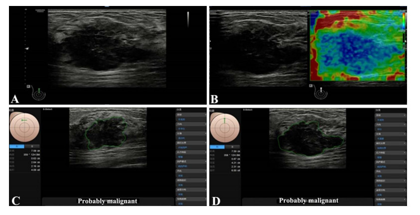
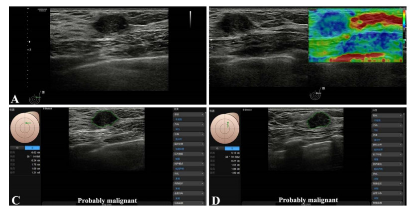
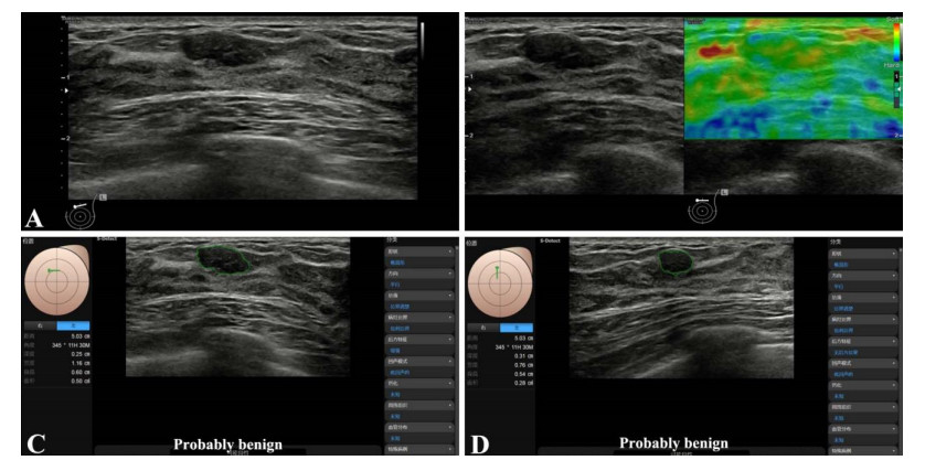
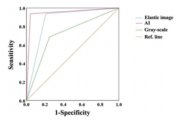
The ultrasound images of 40 patients who underwent ultrasound examination in our hospital were collected. The conventional ultrasound images, elastic images, and S-Detect mode of breast lesions were analyzed. The breast imaging reporting and data system recommended by the American Society of Radiology (BI-RADS) classification for each breast mass was evaluated both by the doctor and AI. The receiver operator characteristics (ROC) curves were drawn to compare the diagnostic efficiency.
Result
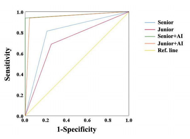
Among the 40 lesions, 16 were benign, and 24 were malignant. The S-Detect AI system had a high diagnostic efficiency for malignant mass, with sensitivity, specificity, and accuracy of 95.8%, 93.8%, and 89.6%. The accuracy of AI was higher than the elastic image and then than the conventional gray-scale image. With the assistance of the S-Detect AI system, the accuracy of BI-RADS classification was improved significantly.
Conclusion
The S-Detect AI system will enhance breast cancer diagnostic accuracy and improve ultrasound examination quality.
- ultrasonography,
- artificial intelligence,
- breast cancer,
- S-Detect technique,
- diagnostic efficiency
Citation: Qun Xia, Yangmei Cheng, Jinhua Hu, Juxia Huang, Yi Yu, Hongjuan Xie, Jun Wang. Differential diagnosis of breast cancer assisted by S-Detect artificial intelligence system[J]. Mathematical Biosciences and Engineering, 2021, 18(4): 3680-3689. doi: 10.3934/mbe.2021184

Related Papers:

Abstract

Objective

Traditional breast ultrasound relies too much on the operation skills of diagnostic doctors, and the repeatability in different doctors was low. This study aimed to evaluate the assistant diagnostic value of S-Detect artificial intelligence (AI) system in differentiating benign from malignant breast masses.

Methods

The ultrasound images of 40 patients who underwent ultrasound examination in our hospital were collected. The conventional ultrasound images, elastic images, and S-Detect mode of breast lesions were analyzed. The breast imaging reporting and data system recommended by the American Society of Radiology (BI-RADS) classification for each breast mass was evaluated both by the doctor and AI. The receiver operator characteristics (ROC) curves were drawn to compare the diagnostic efficiency.

Result

Among the 40 lesions, 16 were benign, and 24 were malignant. The S-Detect AI system had a high diagnostic efficiency for malignant mass, with sensitivity, specificity, and accuracy of 95.8%, 93.8%, and 89.6%. The accuracy of AI was higher than the elastic image and then than the conventional gray-scale image. With the assistance of the S-Detect AI system, the accuracy of BI-RADS classification was improved significantly.

Conclusion

The S-Detect AI system will enhance breast cancer diagnostic accuracy and improve ultrasound examination quality.

References

[1]	R. Singh, S. V. S. Deo, E. Dhamija, S. Mathur, S. Thulkar, To Evaluate the Accuracy of Axillary Staging Using Ultrasound and Ultrasound-Guided Fine-Needle Aspiration Cytology (USG-FNAC) in Early Breast Cancer Patients-a Prospective Study, Indian J. Surg. Oncol., 11 (2020), 726-734. doi: 10.1007/s13193-020-01222-3
[2]	I. González-Huebra, A. Elizalde, A. García-Baizán, M. Calvo, A. Ezponda, F. Martínez-Regueira, et al., Is it worth to perform preoperative MRI for breast cancer after mammography, tomosynthesis and ultrasound?, Magn. Reson. Imag., 57 (2019), 317-322. doi: 10.1016/j.mri.2018.12.005
[3]	Y. Huang, F. Li, J. Han, C. Peng, Q. Li, L. Cao, et al., Shear wave elastography of breast lesions: quantitative analysis of elastic heterogeneity improves diagnostic performance, Ultrasound Med. Biol., 45 (2019), 1909-1917. doi: 10.1016/j.ultrasmedbio.2019.04.019
[4]	M. Di Segni, V. de Soccio, V. Cantisani, G. Bonito, A. Rubini, G. Di Segni, et al., Automated classification of focal breast lesions according to S-detect: validation and role as a clinical and teaching tool, J. Ultrasound, 21 (2018), 105-118. doi: 10.1007/s40477-018-0297-2
[5]	T. V. Bartolotta, A. A. M. Orlando, L. Spatafora, M. Dimarco, C. Gagliardo, A. Taibbi, S-Detect characterization of focal breast lesions according to the US BI RADS lexicon: a pictorial essay, J. Ultrasound, 23 (2020), 207-215. doi: 10.1007/s40477-020-00447-w
[6]	T. V. Bartolotta, A. A. M. Orlando, M. L. Di Vittorio, F. Amato, M. Dimarco, D. Matranga, et al., S-Detect characterization of focal solid breast lesions: a prospective analysis of inter-reader agreement for US BI-RADS descriptors, J. Ultrasound, 5 (2020), 1-8.
[7]	R. M. Jales, M. T. Dória, K. P. Serra, M. M. Miranda, C. A. Menossi, K. Schumacher, et al., Power Doppler Ultrasonography and Shear Wave Elastography as Complementary Imaging Methods for Suspected Local Breast Cancer Recurrence, J. Ultrasound Med., 37 (2018), 1493-1501. doi: 10.1002/jum.14493
[8]	R. Guo, G. Lu, B. Qin, B. Fei, Ultrasound Imaging Technologies for Breast Cancer Detection and Management: A Review, Ultrasound Med. Biol., 44 (2018), 37-70. doi: 10.1016/j.ultrasmedbio.2017.09.012
[9]	J. Geisel, M. Raghu, R. Hooley, The role of ultrasound in breast cancer screening: the case for and against ultrasound, Semin Ultrasound CT MR, 39 (2018), 25-34. doi: 10.1053/j.sult.2017.09.006
[10]	J. Y. Wu, Z. Z. Zhao, W. Y. Zhang, M. Liang, B. Ou, H. Y. Yang, et al., Computer-aided diagnosis of solid breast lesions with ultrasound: factors associated wth false-negative and false-positive results, J. Ultrasound Med., 38 (2019), 3193-3202. doi: 10.1002/jum.15020
[11]	A. S. Tagliafico, M. Piana, D. Schenone, R. Lai, A. M. Massone, N. Houssami, Overview of radiomics in breast cancer diagnosis and prognostication, Breast, 49 (2020), 74-80. doi: 10.1016/j.breast.2019.10.018
[12]	K. Kim, M. K. Song, E. K. Kim, J. H. Yoon, Clinical application of S-Detect to breast masses on ultrasonography: a study evaluating the diagnostic performance and agreement with a dedicated breast radiologist, Ultrasonography, 36 (2017), 3-9. doi: 10.14366/usg.16012
[13]	E. Cho, E. K. Kim, M. K. Song, J. H. Yoon, Application of computer-aided diagnosis on breast ultrasonography: evaluation of diagnostic performances and agreement of radiologists according to different levels of experience, J. Ultrasound Med., 37 (2018), 209-216. doi: 10.1002/jum.14332
[14]	J. H. Choi, B. J. Kang, J. E. Baek, H. S. Lee, S. H. Kim, Application of computer-aided diagnosis in breast ultrasound interpretation: improvements in diagnostic performance according to reader experience, Ultrasonography, 37 (2018): 217-225. doi: 10.14366/usg.17046
[15]	W. H. Yuan, A. F. Li, Y. H. Chou, H. C. Hsu, Y. Y. Chen, Clinical and ultrasonographic features of male breast tumors: A retrospective analysis, PLoS One, 13 (2018), e0194651. doi: 10.1371/journal.pone.0194651
[16]	S. H. Yeo, G. R. Kim, S. H. Lee, W. K. Moon, Comparison of ultrasound elastography and color doppler ultrasonography for distinguishing small triple-negative nreast cancer from fibroadenoma, J. Ultrasound Med., 37 (2018), 2135-2146. doi: 10.1002/jum.14564
[17]	A. Vourtsis, Three-dimensional automated breast ultrasound: Technical aspects and first results, Diagn. Interv. Imaging, 100 (2019), 579-592. doi: 10.1016/j.diii.2019.03.012
[18]	D. A. Spak, J. S. Plaxco, L. Santiago, M. J. Dryden, B. E. Dogan, BI-RADS(®) fifth edition: A summary of changes, Diagn. Interv. Imaging, 98 (2017), 179-190. doi: 10.1016/j.diii.2017.01.001
[19]	X. X. Qu, Y. Song, Y. H. Zhang, H. M. Qing, Value of ultrasonic elastography and conventional ultrasonography in the differential diagnosis of non-mass-like breast lesions, Ultrasound Med. Biol., 45 (2019), 1358-1366. doi: 10.1016/j.ultrasmedbio.2019.01.020
[20]	B. L. Niell, P. E. Freer, R. J. Weinfurtner, E. K. Arleo, J. S. Drukteinis, Screening for breast cancer, Radiol. Clin. North Am., 55 (2017), 1145-1162. doi: 10.1016/j.rcl.2017.06.004
[21]	F. Valdora, N. Houssami, F. Rossi, M. Calabrese, A. S. Tagliafico, Rapid review: radiomics and breast cancer, Breast Cancer Res. Treat., 169 (2018), 217-229. doi: 10.1007/s10549-018-4675-4
[22]	F. Taskin, Y. Durum, A. Soyder, A. Unsal, Review and management of breast lesions detected with breast tomosynthesis but not visible on mammography and ultrasonography, Acta. Radiol., 58 (2017), 1442-1447. doi: 10.1177/0284185117710681

Reader Comments

your name:*

Email:*
© 2021 the Author(s), licensee AIMS Press. This is an open access article distributed under the terms of the Creative Commons Attribution License (http://creativecommons.org/licenses/by/4.0)