Bone remodeling platforms: Understanding the need for multicellular lab-on-a-chip systems and predictive agent-based models

Sharon L. Truesdell; Marnie M. Saunders

doi:10.3934/mbe.2020063

Mathematical Biosciences and Engineering, 2020, 17(2): 1233-1252. doi: 10.3934/mbe.2020063. Opinion paper Special Issues

Export file:

Format

RIS(for EndNote,Reference Manager,ProCite)
BibTex
Text

Content

Citation Only
Citation and Abstract

Bone remodeling platforms: Understanding the need for multicellular lab-on-a-chip systems and predictive agent-based models

Sharon L. Truesdell, Marnie M. Saunders

The Bone Biomechanics and Mechanobiology Lab, Department of Biomedical Engineering, The University of Akron, Akron, OH, USA

Received: , Accepted: , Published:

Special Issues: Recent Advances in Biomedical and Mechanical Engineering and Related Sciences

Abstract Full Text(HTML) Figure/Table Related pages

The purpose of this paper is to emphasize the need for more complex bone remodeling platforms that allow for investigations of intricate multicellular interactions that regulate this process. We discuss the efforts we have taken to develop lab-on-a-chip systems for bone remodeling and the motivation for pursuing more advanced multicellular models. Further, we discuss mathematical modeling opportunities that will allow experimental results to extend beyond the set laboratory conditions. We advocate for the development of an agent-based model comprised of multiple cellular automata of each bone cell type. In total, this work requires a combination of techniques from bone biology, microfluidics, cell mechanobiology, mechanics, and mathematical modeling. Thus, significant advancements within the field will require a collective contribution from a variety of research laboratories.

Figure/Table

Supplementary

Article Metrics

Keywords: bone remodeling; lab-on-a-chip; agent-based models; cellular automata; mechanotransduction; conditioned medium

Citation: Sharon L. Truesdell, Marnie M. Saunders. Bone remodeling platforms: Understanding the need for multicellular lab-on-a-chip systems and predictive agent-based models. Mathematical Biosciences and Engineering, 2020, 17(2): 1233-1252. doi: 10.3934/mbe.2020063

References:

1. B. Clarke, Normal bone anatomy and physiology, J. Am. Soc. Nephrol., 3 (2008), S131-S139.
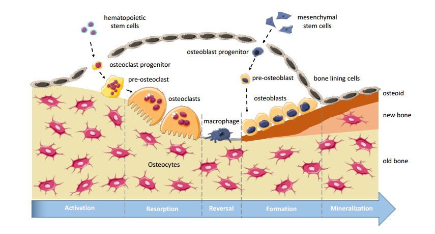
2. J. Kenkre and J. Bassett, The bone remodelling cycle, Ann. Clin. Biochem., 55 (2018), 308-327.
3. L. G. Raisz, Physiology and pathophysiology of bone remodeling, Clin. Chem., 45 (1999), 1353-1358.
4. D. J. Hadjidakis and I. I. Androulaskis, Bone remodeling, Ann. N. Y. Acad. Sci, 1092 (2006), 385-396.
5. E. L. George, S. L. Truesdell, S. L. York, et al., Lab-on-a-chip platforms for quantification of multicellular interactions in bone remodeling, Exp. Cell Res., 365 (2018), 106-118.
6. W. Zhang, C. Green and N. S. Stott, Bone morphogenetic protein-2 modulation of chondrogenic differentiation in vitro involves gap junction-mediated intercellular communication, J. Cell Physiol., 193 (2002), 233-243.
7. J. Ilvesaro, K. Väänänen and J. Tuukkanen, Bone-resorbing osteoclasts contain gap-junctional connexin-43, J. Bone Miner. Res., 15 (2000), 919-926.
8. S. H. Park, W. Y. Sim, B. H. Min, et al., Chip-based comparison of the osteogenesis of human bone marrow- and adipose tissue-derived mesenchymal stem cells under mechanical stimulation, PLoS ONE, 7 (2012), e46689.
9. Y. Zhang, Z. Gazit, G. Pelled, et al., Patterning osteogenesis by inducible gene expression in microfluidic culture systems, Integr. Biol., 3 (2010), 39-47.
10. B. J. Taylor, A. Howell, K. A. Martin, et al., A lab-on-chip for malaria diagnosis and surveillance, Malar. J., 13 (2014), 179.
11. S. Wang, A. Ip, F. Xu, et al., Development of a microfluidic system for measuring HIV-1 viral load, Proc. SPIE, 7666 (2010), 76661H.
12. M. Wheeler and M. Rubessa, Integration of microfluidics and mammalian IVF, Mol. Hum. Reprod., 23 (2016), 248-256.
13. E. K. Sackmann, A. L. Fulton and D. J. Beebe, The present and future role of microfluidics in biomedical research, Nature, 507 (2014), 181-189.
14. D. Huh, B. D. Matthews, A. Mammoto, et al., Reconstituting organ-level lung functions on a chip, Science, 328 (2010), 1662-1668.
15. R. Baudoin, L. Griscom, M. Monge, et al., Development of a renal microchip for in vitro distal tubule models, Biotechnol. Prog., 23 (2007), 1245-1253.
16. K. J. Jang and K. Y. Suh, A multi-layer microfluidic device for efficient culture and analysis of renal tubular cells, Lab Chip, 10 (2010), 36-42.
17. L. L. Bischel, E. W. Young, B. R. Mader, et al., Tubeless microfluidic angiogenesis assay with three-dimensional endothelial-lined microvessels, Biomaterials, 34 (2013), 1471-1477.
18. M. Tsai, A. Kita, J. Leach, et al., In vitro modeling of the microvascular occlusion and thrombosis that occur in hematologic diseases using microfluidic technology, J. Clin. Invest., 122 (2012), 408-418.
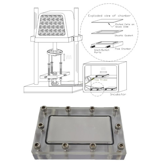
19. M. M. Saunders, Lab-on-a-chip (LOC) for biomimetic bone remodeling, (2018), US Pat. Appl., 1151.
20. K. S. Shah, S. L. York, P. Sethu, et al. Developing a microloading platform for applications in mechanotransduction research, Mechanics of Biological Systems and Materials, Volume 5, Conference Proceedings of the Society for Experimental Mechanics Series, New York: Springer International Publishing, (2013), pp. 197-205.
21. S. L. York, A. R. Arida, K. S. Shah, et al., Osteocyte characterization on polydimethylsiloxane substrates for microsystems applications, J. Biomim. Biomater. Tissue Eng., 16 (2012), 27-42.
22. S. L. York, J. D. King, A. S. Pietros, et al. Development of a microloading platform for in vitro mechanotransduction studies, Mechanics of Biological Systems and Materials, Volume 7, Conference Proceedings of the Society for Experimental Mechanics Series, New York: Springer International Publishing, (2015), pp. 53-59.
23. S. L. York, P. Sethu and M. M. Saunders, In vitro osteocytic microdamage and viability quantification using a microloading platform, Med. Eng. Phys., 38 (2016), 1115-1122.
24. J. D. King, S. L. York and M. M. Saunders, Design, fabrication and characterization of a pure uniaxial microloading system for biologic testing, Med. Eng. Phys., 38 (2016), 411-416.
25. S. L. Truesdell, E. L. George, C. E. Seno, et al., 3D printed loading device for inducing cellular mechanotransduction via matrix deformation, Exp. Mech., 59 (2019), 1223-1232.
26. J. D. King, D. Hayes, K. Shah, et al. Development of a multi-strain profile for cellular mechanotransduction testing, Mechanics of Biological Systems and Materials, Volume 7, Conference Proceedings of the Society for Experimental Mechanics Series, New York: Springer International Publishing, (2015), pp. 61-67.
27. S. L. York, P. Sethu and M. M. Saunders, Impact of gap junctional intercellular communication on MLO-Y4 sclerostin and soluble factor expression, Ann. Biomed. Eng., 44 (2016), 1170-1180.
28. J. M. Delaisse, The reversal phase of the bone-remodeling cycle: Cellular prerequisites for coupling resorption and formation, Bonekey Rep., 3 (2014), 561.
29. N. A. Sims and T. J. Martin, Coupling the activities of bone formation and resorption: A multitude of signals within the basic multicellular unit, Bonekey Rep., 3 (2014), 481.
30. R. Hambli, H. Katerchi, C. L. Benhamou, et al., Multiscale methodology for bone remodelling simulation using coupled finite element and neural network computation, Biomech. Model. Mechanobiol., 10 (2011), 133-145.
31. S. Ilic, K. Hackl and R. Gilbert, Application of the multiscale FEM to the modeling of cancellous bone, Biomech. Model. Mechanobiol., 9 (2010), 87-102.
32. M. D. Ryser, N. Nigam and S. V. Komarova, Mathematical modeling of spatio-temporal dynamics of a single bone multicellular unit, J. Bone Miner. Res., 24 (2009), 860-870.
33. S. Scheiner, P. Pivonka and C. Hellmich, Coupling systems biology with multiscale mechanics, for computer simulations of bone remodeling, Comput. Methods Appl. Mech. Eng., 254 (2013), 181-196.
34. V. Lemaire, F. L. Tobin, L. D. Greller, et al., Modeling the interactions between osteoblast and osteoclast activities in bone remodeling, J. Theor. Biol., 229 (2004), 293-309.
35. P. Pivonka and S. V. Komarova, Mathematical modeling in bone biology: from intracellular signaling to tissue mechanics, Bone, 47 (2010), 181-189.
36. S. A. Colopy, J. Benz-Dean, J. G. Barrett, et al., Response of the osteocyte syncytium adjacent to and distant from linear microcracks during adaptation to cyclic fatigue loading, Bone, 35 (2004), 881-891.
37. J. G. Hazenberg, M. Freeley, E. Foran, et al., Microdamage: A cell transducing mechanism based on ruptured osteocyte processes, J. Biomech., 39 (2006), 2096-2103.
38. O. Verborgt, G. J. Gibson and M. B. Schaffler, Loss of osteocyte integrity in association with microdamage and bone remodeling after fatigue in vivo, J. Bone Miner. Res., 15 (2000), 60-67.
39. G. K. Van Scoy, E. L. George, F. Opoku Asantewaa, et al., A cellular automata model of bone formation, Math. Biosci., 286 (2017), 58-64.
40. J. Eberhard, Y. Efendiev, R. Ewing, et al., Coupled cellular models for biofilm growth and hydrodynamic flow in a pipe, Int. J. Multiscale Compt. Eng., 3 (2005), 499-516.
41. D. G. Mallet and L. G. De Pillis, A cellular automata model of tumor-immune system interactions, J. Theor. Biol., 239 (2006), 334-350.
42. A. Prieto-Langarica, H. Kojouharov, B. Chen-Charpentier, et al., A cellular automata model of infection control on medical implants, Appl. Appl. Math., 6 (2011), 1-10.
43. R. Bivand, E. Pebesma and V. Gómez Rubio, Applied spatial data analysis with R, 2013.
44. P. A. Moran, Notes on continuous stochastic phenomena, Biometrika, 37 (1950), 17-23.

show all references

Reader Comments

your name: * your email: *

Download full text in PDF

Associated material

Metrics