


Citation: Raimund BÜrger, Gerardo Chowell, Elvis GavilÁn, Pep Mulet, Luis M. Villada. Numerical solution of a spatio-temporal gender-structured model for hantavirus infection in rodents[J]. Mathematical Biosciences and Engineering, 2018, 15(1): 95-123. doi: 10.3934/mbe.2018004
| [1] | Raimund Bürger, Gerardo Chowell, Elvis Gavilán, Pep Mulet, Luis M. Villada . Numerical solution of a spatio-temporal predator-prey model with infected prey. Mathematical Biosciences and Engineering, 2019, 16(1): 438-473. doi: 10.3934/mbe.2019021 |
| [2] | Curtis L. Wesley, Linda J. S. Allen, Michel Langlais . Models for the spread and persistence of hantavirus infection in rodents with direct and indirect transmission. Mathematical Biosciences and Engineering, 2010, 7(1): 195-211. doi: 10.3934/mbe.2010.7.195 |
| [3] | Ahmed Alshehri, Saif Ullah . A numerical study of COVID-19 epidemic model with vaccination and diffusion. Mathematical Biosciences and Engineering, 2023, 20(3): 4643-4672. doi: 10.3934/mbe.2023215 |
| [4] | Peter Hinow, Pierre Magal, Shigui Ruan . Preface. Mathematical Biosciences and Engineering, 2015, 12(4): i-iv. doi: 10.3934/mbe.2015.12.4i |
| [5] | Fabrizio Clarelli, Roberto Natalini . A pressure model of immune response to mycobacterium tuberculosis infection in several space dimensions. Mathematical Biosciences and Engineering, 2010, 7(2): 277-300. doi: 10.3934/mbe.2010.7.277 |
| [6] | Elvira Barbera, Giancarlo Consolo, Giovanna Valenti . A two or three compartments hyperbolic reaction-diffusion model for the aquatic food chain. Mathematical Biosciences and Engineering, 2015, 12(3): 451-472. doi: 10.3934/mbe.2015.12.451 |
| [7] | Ziqiang Cheng, Jin Wang . Modeling epidemic flow with fluid dynamics. Mathematical Biosciences and Engineering, 2022, 19(8): 8334-8360. doi: 10.3934/mbe.2022388 |
| [8] | Suman Ganguli, David Gammack, Denise E. Kirschner . A Metapopulation Model Of Granuloma Formation In The Lung During Infection With Mycobacterium Tuberculosis. Mathematical Biosciences and Engineering, 2005, 2(3): 535-560. doi: 10.3934/mbe.2005.2.535 |
| [9] | Ali Moussaoui, Vitaly Volpert . The impact of immune cell interactions on virus quasi-species formation. Mathematical Biosciences and Engineering, 2024, 21(11): 7530-7553. doi: 10.3934/mbe.2024331 |
| [10] | Lin Zhang, Yongbin Ge, Xiaojia Yang . High-accuracy positivity-preserving numerical method for Keller-Segel model. Mathematical Biosciences and Engineering, 2023, 20(5): 8601-8631. doi: 10.3934/mbe.2023378 |
Hantavirus (family Bunyaviridae) is a rodent-borne infectious disease of significant concern as it can generate high case fatality rates in the human population [55]. Transmission of hantavirus from infected rodents, the main known reservoir of the virus, to humans, typically occurs via inhalation of aerosols contaminated by virus shed in excreta, saliva, and urine [36]. Risk of infection with hantavirus in the human population is facilitated by crowding conditions and close proximity to rodent populations. Not surprisingly, the total population at risk for hantavirus infection has increased with urbanization rates. In the Americas, hantavirus represents a public health issue particularly in South American countries including Chile [48]. The great majority of hantavirus cases have been reported in China, however [64,65]. A better understanding of the transmission dynamics of hantavirus in rodent populations has the potential to improve interventions strategies aimed at minimizing the number of infections in the human population.
It is the purpose of this contribution to advance a spatio-temporal compartmental model of hantavirus infection in rodents with a focus on its efficient numerical solution. The total population of rodents is subdivided into males and females (indices m and f), and for each of both subpopulations a variant of the well-known susceptible-exposed-infective-recovered (SEIR) compartmental model [33] is formulated. The compartments of male and female individuals are
| u=(u1,…,u8)T=(Sm,Em,Im,Rm,Sf,Ef,If,Rf)T |
as a function of position
| ∂u∂t+∇⋅Fc(u)=DΔu+s(u), | (1.1) |
supplied with initial and boundary conditions, where the convective fluxes
First of all, it worth mentioning that general references to the spatial spread of infectious diseases include [5,22,38,41,52,60]. The basic assumption of our treatment, namely that all epidemiological compartments are distributed over the whole spatial domain, is opposed to the alternative metapopulation approach that describes spatial structure through the relations between a number of well-identified sub-populations or "patches" (cf., e.g., [3,6,7,18,35,57,58]).
In fact, the description of spatial structure by explicitly specifying the mobilities between "patches" is typical for characterizing the behavior of humans, who usually do not "disperse" in response to environmental stimuli (at least not in the relatively short time scales involved in epidemiological modelling) but undertake directed travels, while a description through a convection-diffusion-reaction mechanism is more suitable for non-human infectious agents such as spores, insects, and bacteria that would disperse. The diffusion mechanism is mostly associated with non-human beings is also supported by the fact that classical treatments of diffusion in ecology only include non-human populations (cf. [41,Ch. 13], [43]). This viewpoint is also assumed, for instance, in [22,Ch. 10]. Other references to the movement of animals and spread of diseases by reaction-diffusion equations include [38,44,51]. Furthermore, the distinction between metapopulation models and continuous in space models is also made in the alternative treatments in Sections 4.3 and 4.4 of Sattenspiel [52] and those by van den Driessche [58] and Wu [61] in the same volume. In the latter, a decisive advantage of the spatially continuous approach, namely its amenability to mathematical analysis is emphasized. Furthermore, a reaction-diffusion system based on the well-known non-spatial SIR model [33] is proposed as a prototype spatio-temporal epidemic model, and the underlying assumptions of variants of reaction-diffusion models are broadly discussed, with particular reference to a seminal case study [29,30,42].
A less common ingredient in mathematical epidemiology is the convective term
Still within the framework of reaction-diffusion systems (but in simpler versions than considered here), a number of qualitative analyses of hantavirus models are available. For instance, Abramson and Kenkre [1] advance a two-equation reaction-diffusion model that is a spatial equation of the well-known susceptible-infectious-susceptible (SIS) model (the assumed population of mice is not structured in any other way), and demonstrate that one single lumped parameter, the carrying capacity, essentially controls the dynamics of the system; moreover a spatial distribution of its value explains the formation and disappearance of "refugia", that is of habitat regions with favorable conditions that influence the spatio-temporal patterns of hantavirus [2,34]. Furthermore, based on the Abramson and Kenkre model [1], Buceta et al. [17] study the the impact of seasonality on hantavirus, with the remarkable result that the alternation of seasons, each of which associated with a constant set of epidemiological parameters, may induce the outbreak of Hantavirus infection even if neither season by itself satisfies the environmental requirements for propagation of the disease [17]. The same group also investigated the effects of intrinsic noise on hantavirus spread [24]. Finally, we mention that more recently the Abramson and Kenkre model was refined to give a stage-dependent model with delay [46], where a new compartment corresponds to virus-free young mice, and the new model consists of three ordinary differential equations with delay, or in its recent spatial version presented in [47], in a reaction-diffusion system with delay (where the diffusion operator is expressed in radial variables).
From a computational point of view, and coming back to our own model (1.1), we mention that IMEX Runge-Kutta (IMEX-RK) schemes play an important role. We therefore briefly provide some background on these methods. Roughly speaking, an IMEX-RK method for a convection-diffusion-reaction equation of the type (1.1) consists of a Runge-Kutta scheme with an implicit discretization of the diffusive term combined with an explicit one for the convective and reactive terms. To introduce the main idea, we consider the problem
| dvdt=Φ∗(v)+Φ(v), | (1.2) |
which is assumed to represent a method-of-lines semi-discretization of (1.1), where
The remainder of this work is organized as follows. The mathematical model is introduced in Section 2, starting from the spatiotemporal balance equations of a gender-structured SEIR model (in Section 2.1). The three variants of convective fluxes
The model for the eight unknowns in
| ∂Sm∂t+∇⋅FSm(Sm,Nf,Nm)=B(Nm,Nf)2−Smd(N)−Sm(βfIf+βmIm), | (2.1a) |
| ∂Em∂t+∇⋅FEm(Em,Nf,Nm)=−Emd(N)+Sm(βfIf+βmIm)−δEm, | (2.1b) |
| ∂Im∂t+∇⋅FIm(Im,Nf,Nm)=δEm−Imd(N)−γmIm, | (2.1c) |
| ∂Rm∂t+∇⋅FRm(Rm,Nf,Nm)=γmIm−Rmd(N), | (2.1d) |
| ∂Sf∂t−∇⋅(μSf∇Sf)=B(Nm,Nf)2−Sfd(N)−Sf(βfIf+βm,fIm), | (2.1e) |
| ∂Ef∂t−∇⋅(μEf∇Ef)=−Efd(N)+Sf(βfIf+βm,fIm)−δEf, | (2.1f) |
| ∂If∂t−∇⋅(μIf∇If)=δEf−Ifd(N)−γfIf, | (2.1g) |
| ∂Rf∂t−∇⋅(μRf∇Rf)=γfIf−Rfd(N), | (2.1h) |
where
| B(Nm,Nf)=2bNmNfNm+Nf, |
where
| d(N)=a+cN, |
where
The fluxes appearing in the lefthand sides of the full spatio-temporal model (2.1) have two components for the male compartments, and one for the female compartments. Several alternative choices of
| FX(X,Nf,Nm)=X(κXV(Nf)−μXV(Nm)), | (2.2) |
where
| FX(X,Nf,Nm)=Xφ(Nm+Nf)(κXV(Nf)−μXV(Nm)), | (2.3) |
where the function
| φ(u)={1−u/Kfor 0≤u≤K,0for u<0 or u>K, | (2.4) |
where
| FX(X,Nf,Nm)=XκXV(Nf)−μX∇X, | (2.5) |
where
The non-local unscaled velocity
| V(w)=∇(w∗η)√1+‖∇(w∗η)‖2, | (2.6) |
where
| (w(⋅,t)∗η)(x)=∫Bε(x)w(y,t)η(x−y)dy=∫R2w(y,t)η(x−y)dy. |
(This definition will be modified slightly for points
| ∇(w∗η)=w∗∇η, | (2.7) |
so that
The non-local velocity function (2.6) was introduced recently in a two-species predator-prey model by Colombo and Rossi [20], for which convergence of a numerical scheme was proved by Rossi and Schleper [50]. The evaluation of this velocity function at
Summarizing, we obtain that the convective fluxes
| Fc(u)=(FSm(Sm,Nf,Nm),FEm(Em,Nf,Nm),FIm(Im,Nf,Nm),FRm(Rm,Nf,Nm),0,0,0,0)T,D=diag(0,0,0,0,μSf,μEf,μIf,μRf), |
when the definition of the fluxes is (2.2) (Model 1) or (2.3), (2.4) (Model 2), and
| Fc(u)=(SmκSmV(Nf),EmκEmV(Nf),ImκImV(Nf),RmκRmV(Nf),0,0,0,0)T,D=diag(μSm,μEm,μIm,μRm,μSf,μEf,μIf,μRf), | (2.8) |
for the definition of the fluxes (2.5) (Model 3). In all cases, the vector of reaction terms
| s1(u)=B(Nm,Nf)2−Smd(N)−Sm(βfIf+βmIm),…,s8(u)=γfIf−Rfd(N). |
The system (2.1) is considered on
| u(x,0)=u0(x),x∈Ω, | (2.9) |
where
| (Fc(u)−D∇u)⋅n=0,x∈∂Ω,t∈(0,T], | (2.10) |
where
Assume that the convective fluxes
| ∂Nm∂t+∇⋅(κmNmV(Nf)−μm∇Nm)=B(Nm,Nf)2−Nmd(Nm+Nf), | (2.11a) |
| ∂Nf∂t−μfΔNf=B(Nm,Nf)2−Nfd(Nm+Nf). | (2.11b) |
This model is similar to the non-local predator-prey model recently analyzed by Colombo and Rossi [20]. In fact, their model is precisely recovered if we identify
We take
We discretize
| vℓ,i,j(t)≈uℓ(xi,yj,t),i,j=1,…,M,ℓ=1,…,8 |
given by
| v′=−∇h⋅˜Fc(v)+Bv+S(v), | (3.1) |
to which suitable implicit-explicit Runge-Kutta (IMEX-RK) schemes will be applied for obtaining the final fully-discrete scheme (see Section 3.4). In this equation
| (Bv)ℓ,i,j=μℓ(Δhvℓ)i,j,i,j=1,…,M,ℓ=1,…,8 | (3.2) |
is the discretization of the diffusion terms. Notice that we take
| S(v)ℓ,i,j=sℓ(vℓ,i,j),i,j=1,…,M,ℓ=1,…,8, |
with corresponding submatrices
| Sℓ(v)i,j=sℓ(vℓ,i,j). | (3.3) |
We explain the discretization of the convective term appearing in (3.1) in the next two subsections.
We will use the following identity for the implementation that arises from (2.6) if we take into account (2.7):
| V(w)=w∗ν√1+‖w∗ν‖2,ν=(∂η∂x,∂η∂y). | (3.4) |
The convolutions
| (w∗χ)(x)=∫Bε(0)w(x−y)χ(y)dy, |
are calculated approximately on the discrete grid via a composite Newton-Cotes quadrature formula, such as the composite Simpson rule.
Since
| (w∗χ)(xi,yj)=∫rh−rh∫rh−rhw(xi−x,yj−y)χ(x,y)dxdy≈h2r∑p=−rr∑q=−rαpαqw(xi−xp,yj−yq)χ(xp,yq), |
where
| (w∗χ)(xi,yj)≈r∑p=−rr∑q=−rβp,qw(xi−p,yj−q),βp,q=h2αpαqχ(xp,yq). | (3.5) |
The accuracy order of this approximation is given by that of the quadrature rule, e.g., it is fourth-order accurate for the composite Simpson rule. Consequently, the approximation (3.5) for
| (w∗χ)(xi,yj)≈(W∗hβ)i,j:=r∑p=−rr∑q=−rβp,qw[i−p]M,[j−q]M, | (3.6) |
where we define
| [i]M:={−i+1for −r+1≤i≤0,ifor 1≤i≤M,2M+1−ifor M+1≤i≤M+r. |
The discrete approximation of
| Vh(W)=W∗hν√1+‖W∗hν‖2,ν=(∂η∂x,∂η∂y). |
Since
| ˜wi,j=w[i]M,[j]M,i,j=1,…,2M |
and use the notation
| w[i]M,[j]M=˜w[i]′2M,[j]′2M,i,j=−r+1,…,M+r. |
Therefore (3.6) for
| (W∗hβ)i,j=r∑p=−rr∑q=−rβp,q˜w[i−p]′2M,[j−q]′2M. | (3.7) |
The convolution on the right-hand side of (3.7) can be performed by FFTs applied to the
The convective flux for the
| Fcℓ(u)=uℓ(κℓV(u5+u6+u7+u8)−μℓV(u1+u2+u3+u4)). |
To discretize its divergence
| ˜Fcℓ(v)i,j=vℓ,i,j(κℓVh(v5+v6+v7+v8)i,j−μℓVh(v1+v2+v3+v4)i,j)∈R2. |
Similar arguments are carried out for the other models (2.3) and (2.5).
We introduce the following notation:
| (fxi,j,fyi,j):=˜Fcℓ(v)i,j, |
where we have dropped the
Our purpose is to use a fifth-order WENO finite difference discretization [27,37,53] of
| ∇⋅Fcℓ(u)(xi,yj)≈∇h⋅˜Fc(v)ℓ,i,j:=ˆfxi+1/2,j−ˆfxi−1/2,jh+ˆfyi,j+1/2−ˆfyi,j−1/2h, | (3.8) |
for suitable numerical fluxes
| fx,±i,j=12(fxi,j±αxvℓ,i,j),αx=max |
Likewise, the numerical flux
| \begin{align*} f^{y, \pm}_{i, j}=\frac12\big(f^{y}_{i, j}\pm \alpha^{y} v_{\ell, i, j} \big),\;\; \alpha^{y}=\max\limits_{i, j} |{\boldsymbol{V}}_{h}^y(\boldsymbol{v})_{i, j}|. \end{align*} |
If
| \begin{align*} \hat f^{x}_{i+1/2, j}&=\mathcal{R}^{+} \bigl( f^{x, +}_{i-2:i+2, j} \bigr) +\mathcal{R}^{-} \bigl( f^{x, -}_{i-1:i+3, j}\bigr), \\ \hat f^{y}_{i, j+1/2}&=\mathcal{R}^{+} \bigl( f^{y, +}_{i, j-2:j+2} \bigr) +\mathcal{R}^{-} \bigl( f^{y, -}_{i, j-1:j+3} \bigr), \end{align*} |
where we have used matlab-type notation for submatrices.
We will use IMEX-RK integrators for ODEs, for which only the diffusion term will be treated implicitly, so we rewrite (3.1) as (1.2), where
| \Phi^*(\boldsymbol{v}) := -\nabla_{h}\cdot \widetilde{\boldsymbol{F}}^{\rm{c}}( \boldsymbol{v})+ \boldsymbol{S}(\boldsymbol{v}), \;\;\Phi(\boldsymbol{v}) := \boldsymbol{\mathcal{B}} \boldsymbol{v}. | (3.9) |
For the diffusive part
| \begin{align*} \boldsymbol{D} := \begin{array}{c|c} \boldsymbol{c}&\boldsymbol{A} \\ &\boldsymbol{b}^{\rm{T}} \vphantom{X_X^{X^X}} \end{array},\;\; \hat{\boldsymbol{D}} := \begin{array}{c|c} \hat{\boldsymbol{c}}&\hat{\boldsymbol{A}} \\ & \hat{\boldsymbol{b}}^{\rm{T}} \vphantom{X_{X^X_X}^{X^{X^X}_X}} \end{array}. \end{align*} |
In our simulations, we limit ourselves to the second-order IMEX-RK scheme H-DIRK2(2, 2, 2) that corresponds to
| \begin{align*} \boldsymbol{D} = \begin{array}{c|cc} 1/2&1/2 &0\\ 1/2&0&1/2 \\ &1/2&1/2 \vphantom{\int\limits^.} \end{array}, \;\; \hat{\boldsymbol{D}} = \begin{array}{c|cc} 0&0&0 \\ 1&1&0\\ &1/2&1/2 \vphantom{\int\limits^.} \end{array} \, . \end{align*} |
Alternative choices are provided and discussed in [10,11,45]. If applied to the equation (1.2), the IMEX-RK scheme gives rise to the following algorithm (see [45]).
Algorithm 3.1.
Input: approximate solution vector
for
if
else compute
endif
solve for
| {{\boldsymbol{K}_p} = \Phi^*\bigl(\hat{\boldsymbol{v}}^{(p)}\bigr) + \Phi\bigl( \bar{\boldsymbol{v}}^{(p)} + \Delta t a_{pp} \boldsymbol{K}_p \bigr)} | (3.10) |
endfor
Output: approximate solution vector
To solve the linear equation (3.10) that arises in Algorithm 3.1 for
| \bigl( \boldsymbol{I}-\Delta t a_{pp} \boldsymbol{\mathcal{B}}\bigr) \boldsymbol{K}_{p} =\boldsymbol{b}^{(p)}, \;\;\boldsymbol{b}^{(p)}:= \Phi^*\bigl(\hat{\boldsymbol{v}}^{(p)}\bigr) + \boldsymbol{\mathcal{B}}\bar{\boldsymbol{v}}^{(p)}, | (3.11) |
where
| \begin{split}& \bigl( \boldsymbol{I}_{M\times M}-\Delta t a_{pp} \mu_{\ell}\boldsymbol{\Delta}_h\bigr) (\boldsymbol{K}_{p})_{\ell}\\& = -\nabla_{h}\cdot \tilde{\boldsymbol{F}}_{\ell}^{\rm{c}}( \hat{\boldsymbol{v}}^{(p)})+ \boldsymbol{S}_{\ell}(\hat{\boldsymbol{v}}^{(p)}) + \mu_{\ell}\boldsymbol{\Delta}_h\bar{\boldsymbol{v}}^{(p)}_{\ell}, \;\;\ell=1, \dots, 8, \end{split} | (3.12) |
where
| \begin{align*} \nabla_{h}\cdot \tilde{\boldsymbol{F}}_{\ell}^{\rm{c}}( \hat{\boldsymbol{v}}^{(p)})=0 \;\; \text{for }\;\;\ell\in\{5, 6, 7, 8\} \end{align*} |
(i.e., there is no convection in the models for females); if
| \begin{align*} (\boldsymbol{K}_{p})_{\ell} = -\bigl(\nabla_{h}\cdot \tilde{\boldsymbol{F}}^{\rm{c}}( \hat{\boldsymbol{v}} ^{(p)})\bigr)_{\ell}+ \boldsymbol{S}_{\ell}(\boldsymbol{v}), \end{align*} |
otherwise the solution of (3.12) is performed by Fast Cosine Transforms (due to boundary conditions), which entails a nearly optimal computational cost of
According to [4], we assume that two months (60 days) is the basic time unit,
We wish to present numerical solutions of the different versions of the spatio-temporal model, Models 1 to 3, that can be compared with the example simulated in [4] (that is, by Model 0), and that corresponds to
| (S_{\rm{m}}, E_{\rm{m}}, I_{\rm{m}}, R_{\rm{m}}, S_{\rm{f}}, E_{\rm{f}}, I_{\rm{f}}, R_{\rm{f}})(0) = (450, 10, 10, 10,450, 5, 5, 5) =: \boldsymbol{U}_0^{\rm{T}}. | (4.1) |
(Figure 1 shows the solution of Model 0 for this case.) To this end, we assume that the spatial domain is
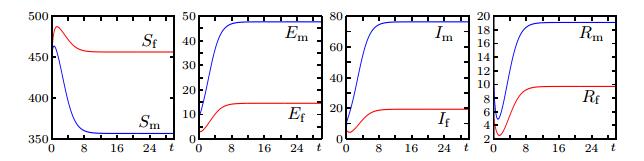 Figure 1. Numerical solution of the ODE version of (2.1), Model 0, for the initial data (4.1).
| \begin{align*} \boldsymbol{u} (\boldsymbol{x}, 0) = \chi_{\Omega_0} (\boldsymbol{x}) \boldsymbol{U}_0, \text{where} \chi_{\Omega_0} (\boldsymbol{x}) = \begin{cases} 1&\text{if }\boldsymbol{x} \in \Omega_0, \\ 0&\text{otherwise, } \end{cases} \end{align*} |
and alternatively Scenario 2, in which we stipulate a "random" distribution by setting
| \boldsymbol{u} (\boldsymbol{x}, 0) = \frac{1}{|\Omega|} \bigl( 1+ r(\boldsymbol{x})\bigr) \boldsymbol{U}_0,\;\; \text{where} \;\; \int_{\Omega} r (\boldsymbol{x}) \, \rm{d} \boldsymbol{x} =0 | (4.2) |
and
A total number of six cases is considered by combining Scenarios 1 and 2 with Models 1, 2 and 3. We always choose
| \mathcal{I} (X) = \mathcal{I} (X, t^n) := h^2 \sum\limits_{i, j=1}^{\rm{N}} X^n_{i, j} \approx \int_{\Omega} X(\boldsymbol{x}, t^n) \, \rm{d} \boldsymbol{x}, | (4.3) |
which represents the approximate total number in
In Figures 2 to 4 we show the numerical solution for
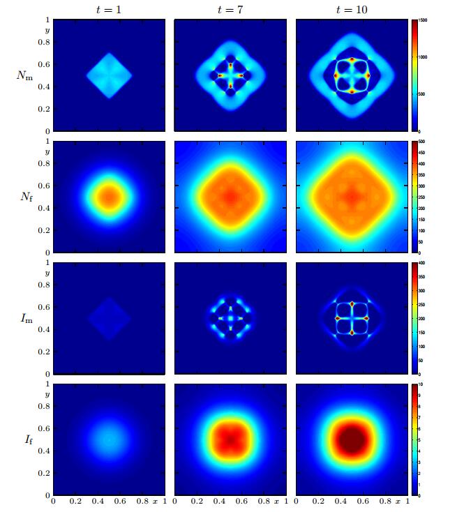 Figure 2. Case 1 (Model 1, Scenario 1): numerical solution for
 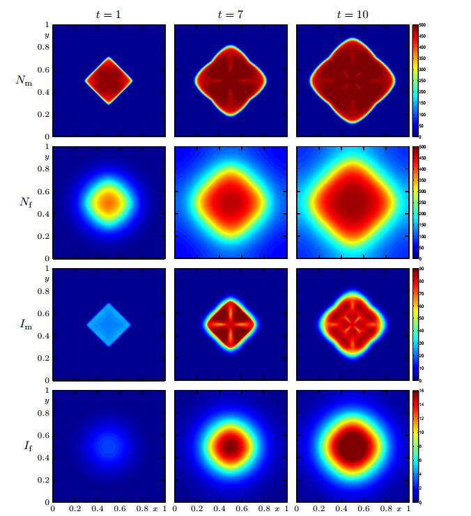 Figure 3. Case 2 (Model 2 with
 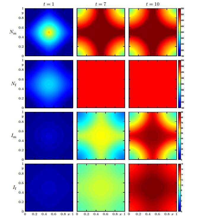 Figure 4. Case 3 (Model 3, Scenario 1): numerical solution for
 The results obtained for Case 1 are in marked contrast to those for Case 2, especially those for
Finally, Figure 5 indicates that Models 1, 2 and 3 lead to quite different numerical results in terms of the integrated quantities (4.3). As mentioned above, the results of Model 3 are similar to those of Model 0. On the other hand, while Models 1 and 2 produce integral results whose order of magnitude for each compartment is similar to that of Model 3, it can be noted that no stationary state is attained at
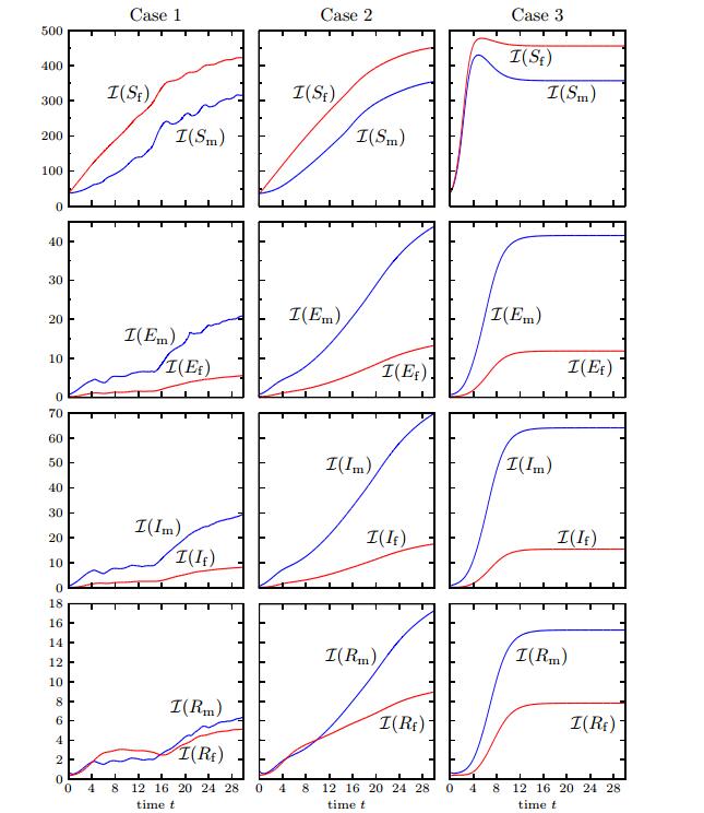 Figure 5. Cases 1-3: integral quantities
 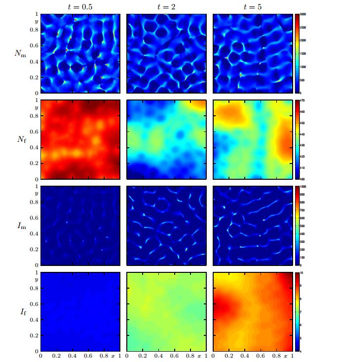 Figure 6. Case 4 (Model 1, Scenario 2): numerical solution for
 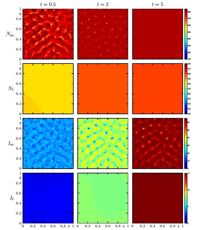 Figure 7. Case 5 (Model 2 with
 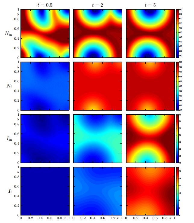 Figure 8. Case 6 (Model 3, Scenario 2): numerical solution for
 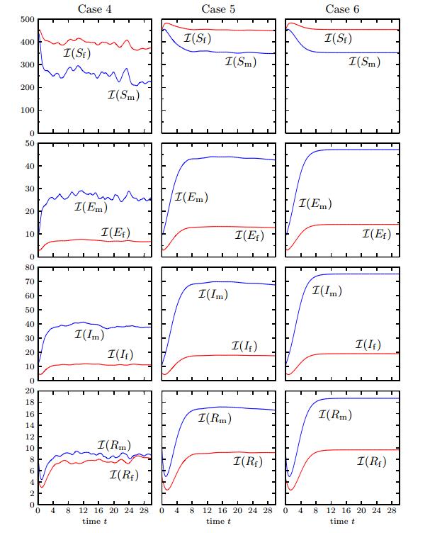 Figure 9. Cases 4-6: integral quantities
 Figures 6 to 9 provide numerical solutions for Scenario 2. The "random" initial datum (4.2) has been chosen to test whether small perturbations would give rise to large-scale regular structures akin to the well-known mechanism of pattern formation (cf., e.g., [38,41]), or rather, the small fluctuations in the initial datum would simply be smoothed out. Figure 6, corresponding to Model 1, illustrates that male individuals aggregate in a kind of filamentous structure, including some marked peaks with
For Cases 4 to 6, we calculate the evolution of Moran's index [25,40,49], denoted here
| \mathsf{I}=\mathsf{I}(X) := \sum\limits_{i, j=1}^{M} \frac{1}{4}Y_{i, j}(Y_{i-1, j}+Y_{i+1, j}+Y_{i, j-1}+Y_{i, j+1}) \biggl/ \sum\limits_{i, j=1}^{M} Y_{i, j}^2, | (4.4) |
where
| Y_{i, j}=X_{i, j}-\frac{1}{M^2}\sum\limits_{p, q=1}^{M}X_{p, q}. | (4.5) |
Overall, the results shown in Figure 10 indicate that a strong spatial autocorrelation (
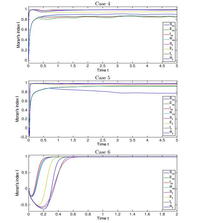 Figure 10. Cases 4-6: Moran's index
 The purpose of this test is to show that the numerical scheme exhibits experimental second order convergence when the solution is smooth. For this purpose, we choose a smooth initial configuration given by
| \begin{align*} X_\rm{m}(x, y, t=0)&=c_X \exp\left(-\frac{1}{2} \bigl((x-3)^6+(y-3)^6 \bigr)\right), \\ X_\rm{f}(x, y, t=0)&=c_X \exp\left(-\frac{1}{2}\bigl((x-7)^6+(y-7)^6\bigr)\right) \end{align*} |
for
We compute approximate
| \tilde{v}^{M}_{\ell, j, k}= \sum\limits_{j_1, k_1=-2}^1 \xi_{j_1}\xi_{k_1}v^{\text{ref}}_{\ell, \bar j-j_1, \bar k - k_1},\;\; \bar j= \left(j-\frac{1}{2}\right)\frac{M_{\text{ref}}}{M}, \;\;\bar k=\left(k-\frac{1}{2}\right)\frac{M_{\text{ref}}}{M}, |
where
The total approximate
| e_M^{\rm{tot}} :=\frac{1}{M^2} \sum\limits_{\ell=1}^8 \sum\limits_{j, k=1}^{M} \bigl|\tilde{v}_{\ell, j, k}^{M}-v_{\ell, j, k}^{M}\bigr|. | (4.6) |
Based on the approximate errors defined by (4.6), we may calculate a numerical order of convergence from pairs of total approximate
| \begin{align*} \theta_M := \log_2 \bigl( e_{M}^{\rm{tot}}/ e_{2M}^{\rm{tot}} \bigr). \end{align*} |
These data are displayed in Table 1. It can be deduced that the errors start diminishing for
|
|
8 | 16 | 32 | 64 | 128 | 256 |
|
|
368.90 | 383.19 | 379.01 | 153.73 | 34.70 | 9.14 |
|
|
-0.05 | 0.02 | 1.30 | 2.15 | 1.92 | - |
 DownLoad: CSV
Climatic changes, e.g.,
due to large periods of rain or of drought, can lead to variation in some parameters,
for example those that influence death and birth rates of the rodent population. To
study the effect of seasonal variability, in this example we identify two different sets
of parameters that can represent two different seasons,
We consider
In Figure 11 we display the numerical solution for Model 3. Roughly speaking we observe that the seasonal alternation in the parameters produces a solution similar to that provided by Model 3 also with a randomly fluctuating initial datum. In Figure 12 we display the solutions for (the ODE) Model 0 and for Model 3. We observe that the seasonal alternation in the parameters generates an oscillatory and bounded solution for each case, and Model 3 displays a smaller amplitude.
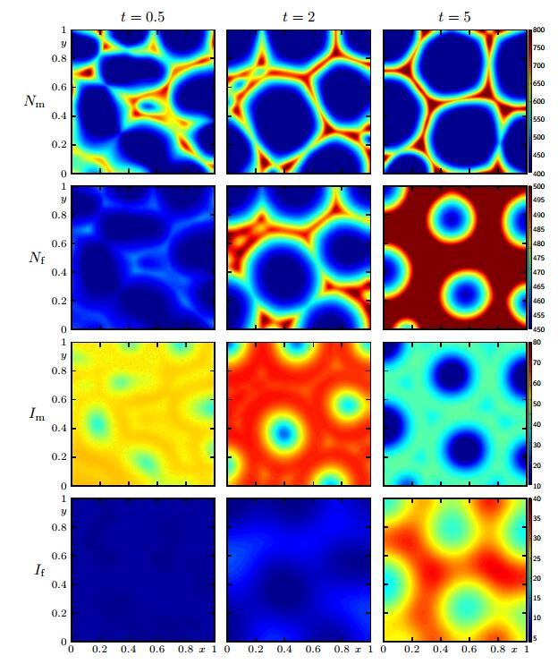 Figure 11. Case 8 (Model 3, Scenario 2, periodic variation of parameters): numerical solution for
 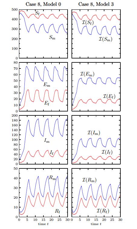 Figure 12. Case 8: (Model 3, Scenario 2, periodic variation of parameters): solutions of Model 0 (left column) and integral quantities
 We have shown that a relatively simple gender-structured spatialtemporal model (2.1) of Hantavirus transmission among rodents with a non-local velocity term (2.6), which arises in each of the Models 1, 2 and 3 defined by (2.2), (2.3) and (2.5), respectively, can yield complex spatial-temporal profiles of disease prevalence (Figures 2 to 8). However, in reality, a number of additional factors can affect the transmission dynamics of Hantavirus infections among rodents. Specifically, the transmission of hantavirus has been associated with land use patterns, elevation, vegetation types [9], as well as variations in temperature, humidity, and rainfall [64]. Moreover, rodent habitat and rodent behavior can be influenced by temperature, precipitation and land use [16]. The growth of rodent populations may also be associated with local temperature, as temperature may affect the pregnancy rate, litter size, birth rate and the survival rate of rodent populations [62]. Further, rodents tend to inhabit highly covered and less disturbed habitats, which are commonly found in agricultural habitats and pastureland habitats [39,63] in order to enhance their reproduction and survival capacity [39].
We plan to conduct further research on the qualitative analysis of the proposed models, or suitable simplifications of them, using analogous techniques to those utilized in [20]. The accuracy of the numerical method proposed in this work is worth to be studied in subsequent works, specially to establish that its order of convergence corresponds to its design order. Although in this work we use a second-order spatial discretization of the Laplacian and a second-order time-stepping, which limit the high-order accuracy of the fifth-order WENO spatial semidiscretization, we plan to perform comparisons with higher-order discretizations of the diffusion operator and time-stepping scheme. More scenarios (initial configuration, parameter calibration) should be explored with these numerical tools in order to obtain and study further spatio-temporal patterns in the simulations. In this sense, among our proposed models, we consider that Model 1 is the most promising one giving rise to interesting spatio-temporal patterns and is worth to be analyzed as in [19,38]. Finally, we wish to expand on the conclusions that can be inferred from
RB is supported by Fondecyt project 1130154; BASAL project CMM, Universidad de Chile and Centro de Investigación en Ingeniería Matemática (CI
| [1] | [ G. Abramson and V. M. Kenkre, Spatiotemporal patterns in the Hantavirus infection Phys. Rev. E 66 (2002), 011912 (5pp). |
| [2] | [ M. A. Aguirre, G. Abramson, A. R. Bishop and V. M. Kenkre, Simulations in the mathematical modeling of the spread of the Hantavirus Phys. Rev. E 66 (2002), 041908 (5pp). |
| [3] | [ L. J. S. Allen,B. M. Bolker,Y. Lou,A. L. Nevai, Asymptotic of the steady states for an SIS epidemic patch model, SIAM J. Appl. Math., 67 (2007): 1283-1309. |
| [4] | [ L. J. S. Allen,R. K. McCormack,C. B. Jonsson, Mathematical models for hantavirus infection in rodents, Bull. Math. Biol., 68 (2006): 511-524. |
| [5] | [ R. M. Anderson,R. M. May, null, Infectious Diseases of Humans: Dynamics and Control, , Oxford Science Publications, 1991. |
| [6] | [ J. Arino, Diseases in metapopulations. In Z. Ma, Y. Zhou and J. Wu (Eds. ), Modeling and Dynamics of Infectious Diseases, Higher Education Press, Beijing, 11 (2009), 64-122. |
| [7] | [ J. Arino,J. R. Davis,D. Hartley,R. Jordan,J. M. Miller,P. van den Driessche, A multi-species epidemic model with spatial dynamics, Mathematical Medicine and Biology, 22 (2005): 129-142. |
| [8] | [ U. Ascher,S. Ruuth,J. Spiteri, Implicit-explicit Runge-Kutta methods for time dependent partial differential equations, Appl. Numer. Math., 25 (1997): 151-167. |
| [9] | [ P. Bi,X. Wu,F. Zhang,K. A. Parton,S. Tong, Seasonal rainfall variability, the incidence of hemorrhagic fever with renal syndrome, and prediction of the disease in low-lying areas of China, Amer. J. Epidemiol., 148 (1998): 276-281. |
| [10] | [ S. Boscarino,R. Bürger,P. Mulet,G. Russo,L. M. Villada, Linearly implicit IMEX Runge-Kutta methods for a class of degenerate convection-diffusion problems, SIAM J. Sci. Comput., 37 (2015): B305-B331. |
| [11] | [ S. Boscarino,F. Filbet,G. Russo, High order semi-implicit schemes for time dependent partial differential equations, J. Sci. Comput., 68 (2016): 975-1001. |
| [12] | [ S. Boscarino,P. G. LeFloch,G. Russo, High-order asymptotic-preserving methods for fully nonlinear relaxation problems, SIAM J. Sci. Comput., 36 (2014): A377-A395. |
| [13] | [ S. Boscarino,G. Russo, On a class of uniformly accurate IMEX Runge-Kutta schemes and applications to hyperbolic systems with relaxation, SIAM J. Sci. Comput., 31 (2009): 1926-1945. |
| [14] | [ S. Boscarino,G. Russo, Flux-explicit IMEX Runge-Kutta schemes for hyperbolic to parabolic relaxation problems, SIAM J. Numer. Anal., 51 (2013): 163-190. |
| [15] | [ F. Brauer,C. Castillo-Chavez, null, Mathematical Models in Population Biology and Epidemiology, Second Ed., Springer, New York, 2012. |
| [16] | [ M. Brummer-Korvenkontio,A. Vaheri,T. Hovi,C. H. von Bonsdorff,J. Vuorimies,T. Manni,K. Penttinen,N. Oker-Blom,J. Lähdevirta, Nephropathia epidemica: Detection of antigen in bank voles and serologic diagnosis of human infection, J. Infect. Dis., 141 (1980): 131-134. |
| [17] | [ J. Buceta, C. Escudero, F. J. de la Rubia and K. Lindenberg, Outbreaks of Hantavirus induced by seasonality Phys. Rev. E 69 (2004), 021908 (9pp). |
| [18] | [ R. Bürger,G. Chowell,P. Mulet,L. M. Villada, Modelling the spatial-temporal progression of the 2009 A/H1N1 influenza pandemic in Chile, Math. Biosci. Eng., 13 (2016): 43-65. |
| [19] | [ R. Bürger,R. Ruiz-Baier,C. Tian, Stability analysis and finite volume element discretization for delay-driven spatio-temporal patterns in a predator-prey model, Math. Comput. Simulation, 132 (2017): 28-52. |
| [20] | [ R. M. Colombo,E. Rossi, Hyperbolic predators versus parabolic preys, Commun. Math. Sci., 13 (2015): 369-400. |
| [21] | [ M. Crouzeix, Une méthode multipas implicite-explicite pour l'approximation des équations d'évolution paraboliques, Numer. Math., 35 (1980): 257-276. |
| [22] | [ O. Diekmann, H. Heesterbeek and T. Britton, Mathematical Tools for Understanding Infectious Disease Dynamics Princeton Series in Theoretical and Computational Biology, Princeton University Press, Princeton, NJ, 2013. |
| [23] | [ R. Donat,I. Higueras, On stability issues for IMEX schemes applied to 1D scalar hyperbolic equations with stiff reaction terms, Math. Comp., 80 (2011): 2097-2126. |
| [24] | [ C. Escudero, J. Buceta, F. J. de la Rubia and K. Lindenberg, Effects of internal fluctuations on the spreading of Hantavirus Phys. Rev. E 70 (2004), 061907 (7pp). |
| [25] | [ S. de Franciscis and A. d'Onofrio, Spatiotemporal bounded noises and transitions induced by them in solutions of the real Ginzburg-Landau model Phys. Rev. E 86 (2012), 021118 (9pp); Erratum, Phys. Rev. E 94 (2016), 0599005(E) (1p). |
| [26] | [ M. Garavello and B. Piccoli, Traffic Flow on Networks. Conservation Laws Models Amer. Inst. Math. Sci. , Springfield, MO, USA, 2006. |
| [27] | [ G. S. Jiang,C.-W. Shu, Efficient implementation of weighted ENO schemes, J. Comput. Phys., 126 (1996): 202-228. |
| [28] | [ P. Kachroo,S. J. Al-Nasur,S. A. Wadoo,A. Shende, null, Pedestrian Dynamics, , Springer-Verlag, Berlin, 2008. |
| [29] | [ A. Källén, Thresholds and travelling waves in an epidemic model for rabies, Nonlin. Anal. Theor. Meth. Appl., 8 (1984): 851-856. |
| [30] | [ A. Källén,P. Arcuri,J. D. Murray, A simple model for the spatial spread and control of rabies, J. Theor. Biol., 116 (1985): 377-393. |
| [31] | [ Y. Katznelson, null, An Introduction to Harmonic Analysis, Third Ed., Cambridge University Press, Cambridge, UK, 2004. |
| [32] | [ C. A. Kennedy,M. H. Carpenter, Additive Runge-Kutta schemes for convection-diffusion-reaction equations, Appl. Numer. Math., 44 (2003): 139-181. |
| [33] | [ W. O. Kermack,A. G. McKendrick, A contribution to the mathematical theory of epidemics, Proc. Roy. Soc. A, 115 (1927): 700-721. |
| [34] | [ N. Kumar, R. R. Parmenter and V. M. Kenkre, Extinction of refugia of hantavirus infection in a spatially heterogeneous environment Phys. Rev. E 82 (2010), 011920 (8pp). |
| [35] | [ T. Kuniya,Y. Muroya,Y. Enatsu, Threshold dynamics of an SIR epidemic model with hybrid and multigroup of patch structures, Math. Biosci. Eng., 11 (2014): 1375-1393. |
| [36] | [ H. N. Liu, L. D. Gao, G. Chowell, S. X. Hu, X. L. Lin, X. J. Li, G. H. Ma, R. Huang, H. S. Yang, H. Tian and H. Xiao, Time-specific ecologic niche models forecast the risk of hemorrhagic fever with renal syndrome in Dongting Lake district, China, 2005-2010, PLoS One, 9 (2014), e106839 (8pp). |
| [37] | [ X.-D. Liu,S. Osher,T. Chan, Weighted essentially non-oscillatory schemes, J. Comput. Phys., 115 (1994): 200-212. |
| [38] | [ H. Malchow,S. V. Petrovskii,E. Venturino, null, Spatial Patterns in Ecology and Epidemiology: Theory, Models, and Simulation, , Chapman & Hall/CRC, Boca Raton, FL, USA, 2008. |
| [39] | [ J. N. Mills,B. A. Ellis,K. T. McKee,J. I. Maiztegui,J. E. Childs, Habitat associations and relative densities of rodent populations in cultivated areas of central Argentina, J. Mammal., 72 (1991): 470-479. |
| [40] | [ P. A. P. Moran, Notes on continuous stochastic phenomena, Biometrika, 37 (1950): 17-23. |
| [41] | [ J. D. Murray, null, Mathematical Biology Ⅱ: Spatial Models and Biomedical Applications, Third Edition, Springer, New York, 2003. |
| [42] | [ J. D. Murray,E. A. Stanley,D. L. Brown, On the spatial spread of rabies among foxes, Proc. Roy. Soc. London B, 229 (1986): 111-150. |
| [43] | [ A. Okubo,S. A. Levin, null, Diffusion and Ecological Problems: Modern Perspectives, Second Edition, Springer-Verlag, New York, 2001. |
| [44] | [ O. Ovaskainen and E. E. Crone, Modeling animal movement with diffusion, in S. Cantrell, C. Cosner and S. Ruan (Eds. ), Spatial Ecology, Chapman & Hall/CRC, Boca Raton, FL, USA, 2009, 63-83. |
| [45] | [ L. Pareschi,G. Russo, Implicit-Explicit Runge-Kutta schemes and applications to hyperbolic systems with relaxation, J. Sci. Comput., 25 (2005): 129-155. |
| [46] | [ J. A. Reinoso and F. J. de la Rubia, Stage-dependent model for the Hantavirus infection: The effect of the initial infection-free period Phys. Rev. E 87 (2013), 042706 (6pp). |
| [47] | [ J. A. Reinoso and F. J. de la Rubia, Spatial spread of the Hantavirus infection Phys. Rev. E 91 (2015), 032703 (5pp). |
| [48] | [ R. Riquelme,M. L. Rioseco,L. Bastidas,D. Trincado,M. Riquelme,H. Loyola,F. Valdivieso, Hantavirus pulmonary syndrome, southern chile, 1995-2012, Emerg. Infect. Dis., 21 (2015): 562-568. |
| [49] | [ C. Robertson, C. Mazzetta and A. d'Onofrio, Regional variation and spatial correlation, Chapter 5 in P. Boyle and M. Smans (Eds. ), Atlas of Cancer Mortality in the European Union and the European Economic Area 1993-1997, IARC Scientific Publication, WHO Press, Geneva, Switzerland, 159 (2008), 91-113. |
| [50] | [ E. Rossi,V. Schleper, Convergence of a numerical scheme for a mixed hyperbolic-parabolic system in two space dimensions, ESAIM Math. Modelling Numer. Anal., 50 (2016): 475-497. |
| [51] | [ S. Ruan and J. Wu, Modeling spatial spread of communicable diseases involving animal hosts, in S. Cantrell, C. Cosner and S. Ruan (Eds. ), Spatial Ecology, Chapman & Hall/CRC, Boca Raton, FL, USA, 2010,293-316. |
| [52] | [ L. Sattenspiel, The Geographic Spread of Infectious Diseases: Models and Applications Princeton Series in Theoretical and Computational Biology, Princeton University Press, 2009. |
| [53] | [ C.-W. Shu,S. Osher, Efficient implementation of essentially non-oscillatory shock-capturing schemes, Ⅱ, J. Comput. Phys., 83 (1988): 32-78. |
| [54] | [ S. W. Smith, Digital Signal Processing: A Practical Guide for Engineers and Scientists. Demystifying technology series: by engineers, for engineers. Newnes, 2003. |
| [55] | [ H. Y. Tian, P. B. Yu, A. D. Luis, P. Bi, B. Cazelles, M. Laine, S. Q. Huang, C. F. Ma, S. Zhou, J. Wei, S. Li, X. L. Lu, J. H. Qu, J. H. Dong, S. L. Tong, J. J. Wang, B. Grenfell and B. Xu, Changes in rodent abundance and weather conditions potentially drive hemorrhagic fever with renal syndrome outbreaks in Xi'an, China, 2005-2012, PLoS Negl. Trop. Dis. , 9 (2015), paper e0003530 (13pp). |
| [56] | [ M. Treiber,A. Kesting, null, Traffic Flow Dynamics, , Springer-Verlag, Berlin, 2013. |
| [57] | [ P. van den Driessche, Deterministic compartmental models: Extensions of basic models, In F. Brauer, P. van den Driessche and J. Wu (Eds. ), Mathematical Epidemiology, SpringerVerlag, Berlin, 1945 (2008), 147-157. |
| [58] | [ P. van den Driessche, Spatial structure: Patch models, In F. Brauer, P. van den Driessche and J. Wu (Eds. ), Mathematical Epidemiology, Springer-Verlag, Berlin, 1945 (2008), 179-189. |
| [59] | [ P. van den Driessche,J. Watmough, Reproduction numbers and sub-threshold endemic equilibria for compartmental models of disease transmission, Math. Biosci., 180 (2002): 29-48. |
| [60] | [ E. Vynnycky,R. E. White, null, An Introduction to Infectious Disease Modelling, , Oxford University Press, 2010. |
| [61] | [ J. Wu, Spatial structure: Partial differential equations models, In F. Brauer, P. van den Driessche and J. Wu (Eds. ), Mathematical Epidemiology, Springer-Verlag, Berlin, 2008,191-203. |
| [62] | [ H. Xiao,X. L. Lin,L. D. Gao,X. Y. Dai,X. G. He,B. Y. Chen, Environmental factors contributing to the spread of hemorrhagic fever with renal syndrome and potential risk areas prediction in midstream and downstream of the Xiangjiang River [in Chinese], Scientia Geographica Sinica, 33 (2013): 123-128. |
| [63] | [ C. J. Yahnke,P. L. Meserve,T. G. Ksiazek,J. N. Mills, Patterns of infection with Laguna Negra virus in wild populations of Calomys laucha in the central Paraguayan chaco, Am. J. Trop. Med. Hyg., 65 (2001): 768-776. |
| [64] | [ W. Y. Zhang,L. Q. Fang,J. F. Jiang,F. M. Hui,G. E. Glass,L. Yan,Y. F. Xu,W. J. Zhao,H. Yang,W. Liu, Predicting the risk of hantavirus infection in Beijing, People's Republic of China, Am. J. Trop. Med. Hyg., 80 (2010): 678-683. |
| [65] | [ W. Y. Zhang,W. D. Guo,L. Q. Fang,C. P. Li,P. Bi,G. E. Glass,J. F. Jiang,S. H. Sun,Q. Qian,W. Liu,L. Yan,H. Yang,S. L. Tong,W. C. Cao, Climate variability and hemorrhagic fever with renal syndrome transmission in Northeastern China, Environ. Health Perspect, 118 (2010): 915-920. |
| [66] | [ X. Zhong, Additive semi-implicit Runge-Kutta methods for computing high-speed nonequilibrium reactive flows, J. Comput. Phys., 128 (1996): 19-31. |
| 1. | Raimund Bürger, Elvis Gavilán, Daniel Inzunza, Pep Mulet, Luis Miguel Villada, Implicit-Explicit Methods for a Convection-Diffusion-Reaction Model of the Propagation of Forest Fires, 2020, 8, 2227-7390, 1034, 10.3390/math8061034 | |
| 2. | Josephine Davies, Kamalini Lokuge, Kathryn Glass, Routine and pulse vaccination for Lassa virus could reduce high levels of endemic disease: A mathematical modelling study, 2019, 37, 0264410X, 3451, 10.1016/j.vaccine.2019.05.010 | |
| 3. | Alberto d’Onofrio, Malay Banerjee, Piero Manfredi, Spatial behavioural responses to the spread of an infectious disease can suppress Turing and Turing–Hopf patterning of the disease, 2020, 545, 03784371, 123773, 10.1016/j.physa.2019.123773 | |
| 4. | Raimund Bürger, Elvis Gavilán, Daniel Inzunza, Pep Mulet, Luis Miguel Villada, Exploring a Convection–Diffusion–Reaction Model of the Propagation of Forest Fires: Computation of Risk Maps for Heterogeneous Environments, 2020, 8, 2227-7390, 1674, 10.3390/math8101674 | |
| 5. | Yanni Xiao, Yunhu Zhang, Min Gao, Modeling hantavirus infections in mainland China, 2019, 360, 00963003, 28, 10.1016/j.amc.2019.05.009 | |
| 6. | Rinaldo M. Colombo, Elena Rossi, Well‐posedness and control in a hyperbolic–parabolic parasitoid–parasite system, 2021, 147, 0022-2526, 839, 10.1111/sapm.12402 | |
| 7. | Robert R. Parmenter, Gregory E. Glass, Hantavirus outbreaks in the American Southwest: Propagation and retraction of rodent and virus diffusion waves from sky-island refugia, 2022, 36, 0217-9792, 10.1142/S021797922140052X | |
| 8. | Juan Pablo Gutiérrez Jaraa, María Teresa Quezada, Modeling of hantavirus cardiopulmonary syndrome, 2022, 22, 07176384, e002526, 10.5867/medwave.2022.03.002526 | |
| 9. | Asep K. Supriatna, Herlina Napitupulu, Meksianis Z. Ndii, Bapan Ghosh, Ryusuke Kon, Chung-Min Liao, A Mathematical Model for Transmission of Hantavirus among Rodents and Its Effect on the Number of Infected Humans, 2023, 2023, 1748-6718, 1, 10.1155/2023/9578283 |


Figures(12) / Tables(1)

Raimund BÜrger, Gerardo Chowell, Elvis GavilÁn, Pep Mulet, Luis M. Villada. Numerical solution of a spatio-temporal gender-structured model for hantavirus infection in rodents[J]. Mathematical Biosciences and Engineering, 2018, 15(1): 95-123. doi: 10.3934/mbe.2018004

|
|
8 | 16 | 32 | 64 | 128 | 256 |
|
|
368.90 | 383.19 | 379.01 | 153.73 | 34.70 | 9.14 |
|
|
-0.05 | 0.02 | 1.30 | 2.15 | 1.92 | - |
DownLoad: CSV