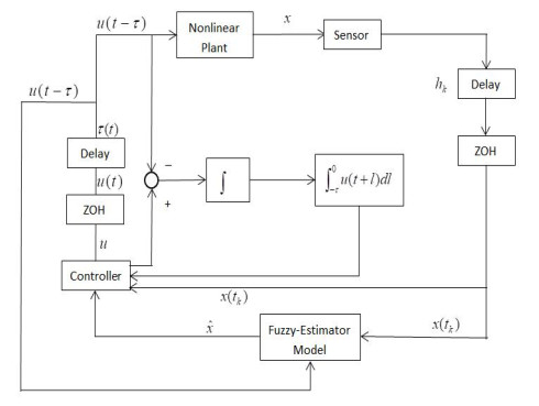
In this paper, an adaptive fuzzy backstepping control strategy is studied for nonlinear nonstrict feedback systems with sampled data and time-varying input delay. Considering the practical application of the proposed control strategy, a time-varying signal transmission delay is investigated. By using fuzzy logic systems to approximate the unknown nonlinear functions, a fuzzy estimator (FE) model is proposed to estimate the states of the nonlinear plant, which is mainly utilized to support information of estimation states for the adaptive fuzzy controller. In the proposed strategy, the constraint between the signal transmission delay and the time-varying input delay is given to ensure the stability of the closed-loop system, and the state vectors are transformed to address the problem of time-varying input delay. By using the backstepping control technique and the information of the FE model, an adaptive fuzzy backstepping controller is designed. The proposed control strategy can guarantee that all signals of the closed-loop system are semi-globally uniformly ultimately bounded. Ultimately, a numerical simulation example is provided to verify the effectiveness of the proposed control method and theory.
Citation: Kunting Yu, Yongming Li. Adaptive fuzzy control for nonlinear systems with sampled data and time-varying input delay[J]. AIMS Mathematics, 2020, 5(3): 2307-2325. doi: 10.3934/math.2020153
In this paper, an adaptive fuzzy backstepping control strategy is studied for nonlinear nonstrict feedback systems with sampled data and time-varying input delay. Considering the practical application of the proposed control strategy, a time-varying signal transmission delay is investigated. By using fuzzy logic systems to approximate the unknown nonlinear functions, a fuzzy estimator (FE) model is proposed to estimate the states of the nonlinear plant, which is mainly utilized to support information of estimation states for the adaptive fuzzy controller. In the proposed strategy, the constraint between the signal transmission delay and the time-varying input delay is given to ensure the stability of the closed-loop system, and the state vectors are transformed to address the problem of time-varying input delay. By using the backstepping control technique and the information of the FE model, an adaptive fuzzy backstepping controller is designed. The proposed control strategy can guarantee that all signals of the closed-loop system are semi-globally uniformly ultimately bounded. Ultimately, a numerical simulation example is provided to verify the effectiveness of the proposed control method and theory.

| [1] | T. Wang, Y. F. Zhang, J. B. Qiu, et al. Adaptive fuzzy backstepping control for a class of nonlinear systems with sampled and delayed measurements, IEEE T. Fuzzy Syst., 23 (2015), 302-312. |
| [2] | L. X. Wang, Adaptive Fuzzy Systems and Control: Design and Stability Analysis, Prentice-Hall, Englewood Cliffs, 1994. |
| [3] | X. H. Su, Z. Liu, G. Y. Lai, et al. Event-triggered adaptive fuzzy control for uncertain strictfeedback nonlinear systems with guaranteed transient performance, IEEE T. Fuzzy Syst., 27 (2019), 2327-2337. |
| [4] | X. M. Zhang, X. K. Liu, Y. Li, Adaptive fuzzy tracking control for nonlinear strict-feedback systems with unmodeled dynamics via backstepping technique, Neurocomputing, IEEE T. Fuzzy Syst., 235 (2017), 182-191. |
| [5] | D. Zhai, L. W. An, J. H. Li, Simplified filtering-based adaptive fuzzy dynamic surface control approach for non-linear strict-feedback systems, IET Control Theory A., 10 (2016), 493-503. |
| [6] | Y. M. Li, X. Min, S. C. Tong, Adaptive fuzzy inverse optimal control for uncertain strict-feedback nonlinear systems, IEEE T. Fuzzy Syst., (2016), In press. |
| [7] | Q. Zhou, C. Wu, P. Shi, Observer-based adaptive fuzzy tracking control of nonlinear systems with time delay and input saturation, Fuzzy Set. Syst., 316 (2017), 49-68. |
| [8] | W. M. Chang, S. C. Tong, Y. M. Li, Adaptive fuzzy backstepping output constraint control of flexible manipulator with actuator saturation, Neur. Comput. Appl., 28 (2017), 1165-1175. |
| [9] | B. Chen, X. P. Liu, S. C. Tong, et al. Observer and adaptive fuzzy control design for nonlinear strict-feedback systems with unknown virtual control coefficients, IEEE T. Fuzzy Syst., 26 (2018), 1732-1743. |
| [10] | Y. M. Li, S. C. Tong, T. S. Li, Hybrid fuzzy adaptive output feedback control design for uncertain MIMO nonlinear systems with time-varying delays and input saturation, IEEE T. Fuzzy Syst., 24 (2016), 841-853. |
| [11] | S. C. Tong, K. K. Sun, S. Sui, AObserver-based adaptive fuzzy decentralized optimal control design for strict-feedback nonlinear large-scale systems, IEEE T. Fuzzy Syst., 26 (2015), 569-584. |
| [12] | H. Q. Wang, B. Chen, C. Lin, Approximation-based adaptive fuzzy control for a class of nonstrict-feedback stochastic nonlinear systems, Sci. China Inform. Sci., 57 (2014), 1-16. |
| [13] | B. Yao, M. Tomizuka, Adaptive robust control of MIMO nonlinear systems in semi-strict feedback forms, Automatica, 37 (2001), 1305-1321. |
| [14] | B. Chen, X. P. Liu, S. Z. S. Ge, et al. Adaptive fuzzy control of a class of nonlinear systems by fuzzy approximation approach, IEEE T. Fuzzy Syst., 20 (2012), 1012-1021. |
| [15] | B. Chen, K. F. Liu, X. P. Liu, et al. Approximation-based adaptive neural control design for a class of nonlinear systems, IEEE T. Cybernetics, 44 (2014), 610-619. |
| [16] | B. Chen, Z. H. Guang, C. Lin, Observer-based adaptive neural network control for nonlinear systems in nonstrict-feedback form, IEEE T. Neur. Net. Lear., 27 (2016), 89-98. |
| [17] | S. C. Tong, Y. M. Li, S. Sui, Adaptive fuzzy tracking control design for SISO uncertain nonstrict feedback nonlinear systems, IEEE T. Cybernetics, 24 (2016), 1141-1454. |
| [18] | S. Yin, P. Shi, H. Y. Yang, Adaptive fuzzy control of strict-feedback nonlinear time-delay systems with unmodeled dynamics, IEEE T. Cybernetics, 46 (2016), 1926-1938. |
| [19] | J. Na, Y. B. Huang, X. Wu, et al. Adaptive finite-time fuzzy control of nonlinear active suspension systems with input delay, IEEE T. Cybernetics, (2019), In press. |
| [20] | H. Y. Li, L. J. Wang, H. P. Du, et al. Adaptive fuzzy backstepping tracking control for strictfeedback systems with input delay, IEEE T. Fuzzy Syst., 25 (2017), 642-652. |
| [21] | B. Niu, L. Li, Adaptive backstepping-based neural tracking control for MIMO nonlinear switched systems subject to input delays, IEEE T. Neur. Net. Lear., 29 (2018), 2638-3644. |
| [22] | Q. Zhou, C. W. Wu, X. J. Jing, et al. Adaptive fuzzy backstepping dynamic surface control for nonlinear input-delay systems, Neurocomputing, 199 (2016), 58-65. |
| [23] | H. Y. Li, X. J. Sun, P. Shi, et al. Control design of interval type-2 fuzzy systems with actuator fault: sampled-data control approach, Inform. Sci., 302 (2015), 1-13. |
| [24] | M. S. Ali, N. Gunasekaran, Q. X. Zhu, State estimation of T-S fuzzy delayed neural networks with Markovian jumping parameters using sampled-data control, Fuzzy Set. Syst., 306 (2017), 87-104. |
| [25] | Y. J. Liu, B. Z. Guo, J. H. Park, et al. Nonfragile exponential synchronization of delayed complex dynamical networks with memory sampled-data control, IEEE T. Neur. Net. Lear., 29 (2018), 118-128. |
| [26] | S. P. Xiao, H. H. Lian, K. Teo, et al. A new Lyapunov functional approach to sampled-data synchronization control for delayed neural networks, J. Franklin I., 335 (2018), 8857-8873. |
| [27] | W. Y. Zhang, J. M. Li, K. Y. Xing, et al. Synchronization for distributed parameter NNs with mixed delays via sampled-data control, Neurocomping, 175 (2016), 265-277. |
| [28] | J. Fu, T. F. Li, T. Y. Chai, et al. Sampled-data-based stabilization of switched linear neutral systems, Automatica, 72 (2016), 92-99. |
| [29] | S. B. Ding, Z. S. Wang, N. N. Rong, et al. Exponential stabilization of memristive neural networks via saturating sampled-data control, IEEE T. Cybernetics, 47 (2017), 3027-3039. |
| [30] | S. Li, C. K. Ahn, Z. R. Xiang, Sampled-data adaptive output feedback fuzzy stabilization for switched nonlinear systems with asynchronous switching, IEEE T. Fuzzy Syst., 27 (2019), 200-205. |
| [31] | W. H. Liu, C. C. Lim, P. Shi, et al. Sampled-data fuzzy control for a class of nonlinear systems with missing data and disturbances, Fuzzy Set. Syst., 306 (2017), 63-86. |
| [32] | Z. H. Qu, Robust Control of Nonlinear Uncertain System, Wiley, New York, 1998. |
| [33] | T. Wang, J. Wu, Y. J. Wang, et al. Adaptive fuzzy tracking control for a class of strict-feedback nonlinear systems with time-varying input delay and full state constrains, IEEE T. Fuzzy Syst., (2019), In press. |
| [34] | X. D. Li, P. Li, Q. G. Wang, Input/output-to-state stability of impulsive switched systems, Syst. Control Lett., 116 (2018), 1-7. |
| [35] | X. Y. Zhang, X. D. Li, J. D. Cao, et al. Design of memory controllers for finite-time stabilization of delayed neural networks with uncertainty, J. Franklin I., 335 (2018), 5394-5413. |
| [36] | I. Stamova, T. Stamov, X. D. Li, Global exponential stability of a class of impulsive cellular neural networks with supremums, Int. J. Adapt. Control., 28 (2014), 1227-1237. |
| [37] | X. Tan, J. Cao, X. D. Li, Leader-following mean square consensus of stochastic multi-agent systems with input delay via event-triggered control, IET Control Theory A., 12 (2017), 229-309. |
Figures(10)

Kunting Yu, Yongming Li. Adaptive fuzzy control for nonlinear systems with sampled data and time-varying input delay[J]. AIMS Mathematics, 2020, 5(3): 2307-2325. doi: 10.3934/math.2020153


 DownLoad: