Nano bio-MOF compounds 6–8 (cobalt argeninate, cobalt asparaginate, and cobalt glutaminate) have been evaluated for successful in vitro drugs adsorption of four drugs, terazosine, telmisartan, glimpiride and rosuvastatin. TGA and PXRD spectra of all these materials in pure form and after drugs adsorption have also been recorded to elaborate the phenomenon of in vitro drugs adsorption in these materials. The amounts of adsorbed drugs and their slow release from all these materials have been monitored by the high performance liquid chromatography (HPLC).
Citation: Tabinda Sattar, Muhammad Athar. Nano bio-MOFs: Showing drugs storage property among their multifunctional properties[J]. AIMS Materials Science, 2018, 5(3): 508-518. doi: 10.3934/matersci.2018.3.508
Related Papers:
[1]
Haifeng Zhang, Jinzhi Lei .
Optimal treatment strategy of cancers with intratumor heterogeneity. Mathematical Biosciences and Engineering, 2022, 19(12): 13337-13373.
doi: 10.3934/mbe.2022625
[2]
Andrei Korobeinikov, Conor Dempsey .
A continuous phenotype space model of RNA virus evolution within a host. Mathematical Biosciences and Engineering, 2014, 11(4): 919-927.
doi: 10.3934/mbe.2014.11.919
[3]
Pedro José Gutiérrez-Diez, Jose Russo .
Design of personalized cancer treatments by use of optimal control problems: The case of chronic myeloid leukemia. Mathematical Biosciences and Engineering, 2020, 17(5): 4773-4800.
doi: 10.3934/mbe.2020261
[4]
Tin Phan, Changhan He, Alejandro Martinez, Yang Kuang .
Dynamics and implications of models for intermittent androgen suppression therapy. Mathematical Biosciences and Engineering, 2019, 16(1): 187-204.
doi: 10.3934/mbe.2019010
[5]
Alexis B. Cook, Daniel R. Ziazadeh, Jianfeng Lu, Trachette L. Jackson .
An integrated cellular and sub-cellular model of cancer chemotherapy and therapies that target cell survival. Mathematical Biosciences and Engineering, 2015, 12(6): 1219-1235.
doi: 10.3934/mbe.2015.12.1219
[6]
Cameron Meaney, Gibin G Powathil, Ala Yaromina, Ludwig J Dubois, Philippe Lambin, Mohammad Kohandel .
Role of hypoxia-activated prodrugs in combination with radiation therapy: An in silico approach. Mathematical Biosciences and Engineering, 2019, 16(6): 6257-6273.
doi: 10.3934/mbe.2019312
[7]
Cassidy K. Buhler, Rebecca S. Terry, Kathryn G. Link, Frederick R. Adler .
Do mechanisms matter? Comparing cancer treatment strategies across mathematical models and outcome objectives. Mathematical Biosciences and Engineering, 2021, 18(5): 6305-6327.
doi: 10.3934/mbe.2021315
[8]
Kangbo Bao .
An elementary mathematical modeling of drug resistance in cancer. Mathematical Biosciences and Engineering, 2021, 18(1): 339-353.
doi: 10.3934/mbe.2021018
[9]
Damilola Olabode, Libin Rong, Xueying Wang .
Stochastic investigation of HIV infection and the emergence of drug resistance. Mathematical Biosciences and Engineering, 2022, 19(2): 1174-1194.
doi: 10.3934/mbe.2022054
[10]
Defne Yilmaz, Mert Tuzer, Mehmet Burcin Unlu .
Assessing the therapeutic response of tumors to hypoxia-targeted prodrugs with an in silico approach. Mathematical Biosciences and Engineering, 2022, 19(11): 10941-10962.
doi: 10.3934/mbe.2022511
Abstract
Nano bio-MOF compounds 6–8 (cobalt argeninate, cobalt asparaginate, and cobalt glutaminate) have been evaluated for successful in vitro drugs adsorption of four drugs, terazosine, telmisartan, glimpiride and rosuvastatin. TGA and PXRD spectra of all these materials in pure form and after drugs adsorption have also been recorded to elaborate the phenomenon of in vitro drugs adsorption in these materials. The amounts of adsorbed drugs and their slow release from all these materials have been monitored by the high performance liquid chromatography (HPLC).
1.
Introduction
The emergence of drug resistance in cancer cell populations during anti-cancer therapies is a major issue that is impeding the treatment of human cancers [1]. Most cancers are shown to develop resistance to targeted therapies or chemotherapies, even highly drug-sensitive tumors may show initial responses but develop resistance gradually in the process of treatment, presenting major challenges to personalized medicine [2,3]. It is confirmed that the emergence of drug resistance in cancer cell population stems from intratumor heterogeneity, that is, the coexistence of cellular populations bearing different genetic or epigenetic alterations within the same individual tumors [4,5]. The interplay between intratumor heterogeneity and the tumor microenvironment drives the emergence of resistance, which can be described by the tumor evolution process. Under environmental pressure, subpopulations of cancer cells expressing phenotypes adapted to the local environment have selective advantages, so that they emerge and expand at the expense of others [6]. The evolutionary adaption is driven by the genetic modifications (e.g., mutations) and perturbations of the tumor microenvironment induced by anti-cancer therapy agents. When cancer undergoes selective pressures imposed by anti-cancer therapy, the more stress-resistant phenotypes emerge and expand, thereby cancer adapts to the pharmacologic pressures and affects clinical outcomes. Therefore, it is important to consider the evolution of tumors in implementation of therapeutic strategies [7,8].
Certain combination therapies are shown to be more effective than single drugs, and some preventive combination therapies could block the emergence of resistance [9,10,11]. The scheduling of combination therapies is important for controlling different cancer cell subpopulations, and the therapies implemented at each clinical time point must be determined in advance carefully. Adaptive strategies targeting different branches of tumor cells with alternating administration of corresponding drugs could foster competition between drug-sensitive and drug-resistant subpopulations [12,13,14]. The goal of adaptive therapy design is to keep a controllable and stable tumor load in cancer treatment by allowing for sensitive cells to survive at a certain level in order to suppress proliferation of the less adapted resistant populations [13,15,16,17,18,19,20].
Mathematical modeling with evolutionary game theory and evolutionary adaptive dynamics has been widely applied for the study of cancer evolution and design of adaptive therapy schedules [14,15,16,17,18,21]. Evolutionary game theory is a general modeling framework to study evolutionary dynamics of frequency-dependent selection among populations [22,23,24,25,26,27]. Individuals with fixed strategies in the population, as players in a game, interact randomly with other individuals. The payoff is interpreted as the fitness which relies on the relative proportions (frequencies) of the different phenotypes in the population. Strategies with higher fitness do well and reproduce faster whereas those with lower fitness do poorly and are outcompeted.
Applying frequency-dependent competition models and evolutionary game theory, West J. et al.[13] explored sequential and concomitant therapy strategies and presented novel multidrug adaptive therapy regimens for metastatic castrate resistant prostate cancer patients, that is, patient-specific therapeutic schedules which drive tumor evolution into cycles of a periodic and controllable loop. Zhang J. et al.[14] integrated evolutionary dynamics into the treatment of metastatic castrate-resistant prostate cancer by an evolutionary game theory model with Lotka-Volterra equations, and explored strategies for the control of tumor progression which showed significant improvement in outcomes in pilot clinical trial. Singh G. et al.[20] investigated the design of adaptive therapy dosage by a Lotka-Volterra based population dynamics model of the drug-sensitive, drug-resistant cells, and transient drug-hybrid state along with phenotypic switching during adaptive therapy. Certain key parameter regimes were identified for effective adaptive therapy, and the importance of intermediate drug-hybrid state in cancer was phenomenologically explained. Gluzman M. et al.[24] proposed a method for systematically optimizing the roles of adaptive policies based on an evolutionary game theory model of cancer dynamics and optimized the total drug usage and time to recovery by solving a Hamilton-Jacobi-Bellman equation.
Basanta D. et al.[9] proposed a general evolutionary game theory framework for tumor cell evolution under the constraints of combination therapies. Applying a more specific version of the general model, the authors explored evolutionary dynamics that how chemotherapy can improve the efficacy of the p53 vaccine for small cell lung cancer. In their model, three different tumor subpopulations are considered, that is, regular tumor cells that are susceptible to both p53 vaccine and chemotherapy (sensitive cells), cells that are resistant to chemotherapy and cells resistant to p53 vaccine. By numerical simulation, the authors showed that the schedule that p53 vaccine is administered first and then change to chemotherapy results in entire chemotherapy-resistant cells, while the schedule that chemotherapy is applied first and then change to the p53 vaccine also leads to entire chemotherapy-resistant cells, driving the susceptible and p53 vaccine-resistant populations toward extinction. However, for the schedule that chemotherapy is applied first and then change to the p53 vaccine, we found that, as the simulation time step is extended to 200, p53 vaccine-resistant cells would emerge again and establish while chemotherapy-resistant population and sensitive population are eradicated. Explanation of this phenomenon needs investigation of the underlying evolutionary dynamics.
In this paper, we investigated the evolution outcomes of tumor composed of sensitive cells, chemotherapy-resistant cells and p53 vaccine-resistant cells different schedules of chemotherapy and p53 vaccine therapy by applying a replicator dynamical model with fitness defined by a payoff matrix generalized from [9]. We further explored the design of adaptive therapy schedules with combination of chemotherapy and p53 vaccine. The rest of this paper is organized as follows. In Section 2, we first presented a generalized replicator dynamical model, and then explored analytically and numerically the existence and local asymptotic stability of equilibria of the model. Furthermore, designs of adaptive therapy schedules based evolutionary velocity and evolutionary absorbing regions were illustrated.
Experimental studies on targeted therapy with BRAF, ALK, or EGFR kinase inhibitors showed that these targeted therapies induces the release of sceretome by drug-sensitive cancer cells, which lead to establishment of a tumor microenvironment that supports the expansion of drug-resistant clones [28]. In Section 3, applying the replicator dynamics similar to the model in Section 2, we explored the influence of this supporting effect to the evolution of cancer cell populations under combination of two targeted therapies, via local stability analysis and numerical simulation. The paper is ended by Section 4, where some discussion and conclusions were presented.
2.
Tumor evolution under chemotherapy and p53 vaccine
2.1. Replicator dynamical model
We considered the evolution dynamics of three subpopulations of tumor cells, that is, regular tumor cells susceptible to both the p53 vaccine and chemotherapy (sensitive cells, S), chemotherapy-resistant cells (C) and p53 vaccine-resistant cells (I). The dynamics and interactions of subpopulations are given by the following replicator equations:
dPCdt=PC(WC−¯W),dPIdt=PI(WI−¯W),dPSdt=PS(WS−¯W).
(2.1)
where PC(t), PI(t) and PS(t) represent the proportion of chemotherapy-resistant cells, p53 vaccine-resistant cells and sensitive cells at time t, respectively, with PC+PI+PS=1; WC, WI and WS indicate the fitness of chemotherapy-resistant cells, p53 vaccine-resistant cells and sensitive cells, respectively; ¯W denotes the average fitness of the entire population. To define the fitness, we assumed the competitive interactions between these three cell types are given by the following payoff matrix:
Here, we assumed as in [9] that chemotherapy-resistant cells and vaccine-resistant cells pay a cost of resistance, cC and cI, respectively; the cost of vaccine to sensitive cells and chemotherapy-resistant cells are dI and αdI, respectively, when it is administered; the cost of chemotherapy to sensitive cells and vaccine-resistant cells are dC and βdC, respectively, when it is applied. Here, α and β represent the extra cost of chemotherapy-resistant cells and vaccine-resistant cells being subjected to the different drugs [9], that is, p53 vaccine and chemotherapy, respectively (α,β>1). We also assumed that sensitive cells and chemotherapy-resistance cells get support from vaccine-resistant cells as the vaccine is applied and as they interact with vaccine-resistant cells [9], respectively, which is represented by a factor γ (0<γ<1). The fitness of the three subpopulations are defined by
where →P=(PC,PI,PS)T. The average fitness is given by
¯W=PCWC+PIWI+PSWS.
(2.3)
The fitness of population can be understood as reproduction rate of the population.
2.2. Stability analysis of equilibria
According the properties of general replicator dynamics [22,23], the system (2.1) is defined on the simplex S3={(PC,PI,PS)|PC+PI+PS=1,0≤PC,PI,PS≤1}, and the edges and the interior of the simplex are invariant, respectively. The system (2.1) has seven types of equilibria Ei(PC,PI,PS), i=1,...,7, given as follows.
(I) The equilibria E1(0,0,1), E2(0,1,0) and E3(1,0,0) always exist.
(II) When dC+γdI<cI+βdC<dC+dI, there exists an equilibrium E4(0,ˉPI,ˉPS), where ˉPI=(dC+dI)−(cI+βdC)dI(1−γ), ˉPS=1−ˉPI=(cI+βdC)−(dC+γdI)dI(1−γ)); vaccine-resistant cells and sensitive cells coexist.
(III) When cC+αγdI<cI+βdC<cC+αdI, there exists an equilibrium E5(˜PC,˜PI,0), where ˜PC=(cI+βdC)−(cC+αγdI)αdI(1−γ), ˜PI=1−˜PC=(cC+αdI)−(cI+βdC)αdI(1−γ); chemotherapy-resistant cells and vaccine-resistant cells coexist.
(IV) When dC+dI=cC+αdI, there exists a line of equilibria E6(ˆPC,0,ˆPS), where ˆPC+ˆPS=1; chemotherapy-resistant cells and sensitive cells coexist.
(V) When dC+γdI<cI+βdC<dC+dI and (cC+αdI)−(cI+βdC)=α[(dC+dI)−(cI+βdC)], there exists a line of equilibria E7(P∗C,P∗I,P∗S), where P∗I=(dC+dI)−(cI+βdC)dI(1−γ), P∗C+P∗S=1−P∗I; chemotherapy-resistant cells, vaccine-resistant cells and sensitive cells coexist.
Next we considered the local stability of these equilibria by linearizing the system (2.1) at the equilibria. The stability of equilibria are shown in the following theorems.
Theorem 2.1.The equilibria E1(0,0,1), E2(0,1,0) and E3(1,0,0) of the system (2.1) always exist and their stability conditions are given as follows:
(1) If dC+dI<min{cC+αdI,cI+βdC,1}, then E1(0,0,1) is LAS;
(2) If cI+βdC<min{cC+αγdI,dC+γdI,1}, then E2(0,1,0) is LAS;
(3) If cC+αdI<min{dC+dI,cI+βdC,1}, then E3(1,0,0) is LAS.
Here, LAS means locally asymptotically stable.
Proof. (1) The Jacobian matrix of the system (2.1) at E1(0,0,1) is given by
The corresponding eigenvalues are λ1=(dC+dI)−(cC+αdI), λ2=(dC+dI)−(cI+βdC), λ3=dC+dI−1. Thus, if dC+dI<min{cC+αdI,cI+βdC,1}, then λi<0, i=1,2,3, which implies that the equilibrium E1(0,0,1) is locally asymptotically stable[29,30].
(2) The Jacobian matrix of the system (2.1) at the equilibrium E2(0,1,0) is
The corresponding eigenvalues are λ1=(cI+βdC)−(cC+αγdI), λ2=(cI+βdC)−1, λ3=(cI+βdC)−(dC+γdI), which are negative if cI+βdC<min{cC+αγdI,dC+γdI,1}. Hence, the equilibrium E2(0,1,0) is locally asymptotically stable if cI+βdC<min{cC+αγdI,dC+γdI,1}.
(3) The Jacobian matrix of the system (2.1) at E3(1,0,0) reads
The corresponding eigenvalues are λ1=(cC+αdI)−1, λ2=(cC+αdI)−(cI+βdC), λ3=(cC+αdI)−(dC+dI). We see that cC+αdI<min{dC+dI,cI+βdC,1} implies λi<0, i=1,2,3, so that the equilibrium E3(1,0,0) is locally asymptotically stable.
Theorem 2.2.For the system (2.1),
(1) If dC+γdI<cI+βdC<dC+dI, the equilibrium E4(0,ˉPI,ˉPS) exists, and furthermore if cI+βdC<1 and α[(dC+dI)−(cI+βdC)]<(cC+αdI)−(cI+βdC), then E4(0,ˉPI,ˉPS) is LAS, where ˉPI=(dC+dI)−(cI+βdC)dI(1−γ), ˉPS=1−ˉPI=(cI+βdC)−(dC+γdI)dI(1−γ);
(2) If cC+αγdI<cI+βdC<cC+αdI, the equilibrium E5(˜PC,˜PI,0) exits, if in addition, cI+βdC<1 and α[(dC+dI)−(cI+βdC)]>(cC+αdI)−(cI+βdC), then E5(˜PC,˜PI,0) is LAS, where ˜PC=(cI+βdC)−(cC+αγdI)αdI(1−γ), ˜PI=1−˜PC=(cC+αdI)−(cI+βdC)αdI(1−γ).
Proof. (1) The fitness of the three subpopulations at the equilibrium E4(0,ˉPI,ˉPS) are given by
One of the corresponding eigenvalues is λ1=¯WC−¯WI=(cI+βdC)−(cC+αdI)+α[(dC+dI))−(cI+βdC)], which is negative if α[(dC+dI)−(cI+βdC)]<(cC+αdI)−(cI+βdC). The other two eigenvalues (λ2,λ3) have negative real parts if the following conditions are satisfied:
respectively, noticing that ˉPI+ˉPS=1, ¯WI=¯WS, ˉPI,ˉPS,dI>0 and 0<γ<1. Hence, ¯WS=1−(cI+βdC)>0 ensures the two eigenvalues λ2 and λ3 have negative real parts. Therefore, if cI+βdC<1, α[(dC+dI)−(cI+βdC)]<(cC+αdI)−(cI+βdC), and the equilibrium E4(0,ˉPI,ˉPS) exists, then it is locally asymptotically stable.
(2) The Jacobian matrix of the system (2.1) at E5(˜PC,˜PI,0) is given by
We see that one corresponding eigenvalue is λ1=˜WS−˜WI=(cI+βdC)−(dC+dI)+1α[(cC+αdI)−(cI+βdC)], so that (cC+αdI)−(cI+βdC)<α[(dC+dI)−(cI+βdC)] implies λ1<0. The other two eigenvalues λ2,λ3 have negative real parts, if
respectively, noticing that ˜PC+˜PI=1, ˜WC=˜WI, ˜PI,˜PC,dI>0 and 0<γ<1. Therefore, ˜WC=1−(cI+βdC)>0 guarantees Re(λi)<0, i=2,3. In summary, if the equilibrium E5(˜PC,˜PI,0) exits, and in addition, cI+βdC<1 and (cC+αdI)−(cI+βdC)<α[(dC+dI)−(cI+βdC)], then E5(˜PC,˜PI,0) is locally asymptotically stable.
Theorem 2.3.If and only if dC+dI=cC+αdI, there exists a line of equilibria, E6(ˆPC,0,ˆPS), where ˆPC+ˆPS=1, and they are locally stable if cC+αdI<min{cI+βdC,1}.
Proof. The fitness of the subpopulations at the equilibrium E6(ˆPC,0,ˆPS) are
ˆWC=1−cC−αdI,ˆWI=1−cI−βdC,ˆWS=1−dC−dI.
Note that ˆWC=ˆWS, if E6(ˆPC,0,ˆPS) exists. The Jacobian matrix of the system (2.1) at E6(ˆPC,0,ˆPS) is given by
The corresponding eigenvalues are λ1=0, λ2=ˆWI−ˆWC=(cC+αdI)−(cI+βdC), λ3=−ˆWC=(cC+αdI)−1. Hence, if cC+αdI<min{cI+βdC,1}, then λ2,λ3<0, so that E6(ˆPC,0,ˆPS) is locally stable when it exists (shown numerically in the next subsection).
Theorem 2.4.If dC+γdI<cI+βdC<dC+dI and (cC+αdI)−(cI+βdC)=α[(dC+dI)−(cI+βdC)], there exists a line of equilibria E7(P∗C,P∗I,P∗S), where P∗I=(dC+dI)−(cI+βdC)dI(1−γ), P∗C+P∗S=1−P∗I; they are locally stable if cI+βdC<1.
Proof. The Jacobian matrix of the system (2.1) at E7(P∗C,P∗I,P∗S) reads
where a=α(1−γ)dIP∗CP∗I+(1−γ)dIP∗IP∗S−P∗CW∗−P∗SW∗. The two similar matrices J7 and J∗ have the same eigenvalues, one of which is λ1=0. The real parts of the other two eigenvalues λ2,λ3 are negative as the following conditions hold:
respectively, where P∗C,P∗I,P∗S,α,dI>0 and 0<γ<1. Therefore, W∗=1−cI−βdC>0 permits the other two eigenvalues have negative real parts, and the equilibrium E7(P∗C,P∗I,P∗S) is locally stable (shown numerically in the next subsection), where P∗I=(dC+dI)−(cI+βdC)dI(1−γ), P∗C+P∗S=1−P∗I.
The conditions for existence and local stability of the equilibria Ei, i=1,...,7, were summarized in Table 1, with introduction of the notations fC:=cC+αdI, fI:=cI+βdC, fS:=dC+dI, f∗C:=cC+γαdI and f∗S:=dC+γdI.
Table 1.
The conditions for existence and local asymptotic stability of equilibria Ei, i=1,...,7. Here, fC:=cC+αdI, fI:=cI+βdC, fS:=dC+dI, f∗C:=cC+γαdI, and f∗S:=dC+γdI.
Equilibria Ei(PC,PI,PS)
Existence conditions
LAS conditions
E1(0,0,1)
Always
fS<min{fC,fI,1}
E2(0,1,0)
Always
fI<min{f∗C,f∗S,1}
E3(1,0,0)
Always
fC<min{fS,fI,1}
E4(0,¯PI,¯PS)
f∗S<fI<fS
fI<1, α(fS−fI)<fC−fI
E5(~PC,~PI,0)
f∗C<fI<fC
fI<1, fC−fI<α(fS−fI)
E6(^PC,0,^PS)
fS=fC
fS<min{fI,1}*
E7(P∗C,P∗I,P∗S)
f∗S<fI<fS,fC−fI=α(fS−fI)
fI<1*
* Note: The equilibria E6 and E7 are locally stable, but not asymptotically stable.
Notice that the existence and local stability of the evolutionary stable points Ei, i=1,...,7, are mutually exclusive. Here, we explain some of them, except for the obvious ones. For example, E1(0,0,1) and E5(˜PC,˜PI,0) cannot be bistable: The existence condition of E5, fI<fC, and its LAS condition, fC−fI<α(fS−fI), together imply that fI<fS, under which, E1 is unstable. Similarly, E3(0,0,1) and E4(0,¯PI,¯PS) (or E7(P∗C,P∗I,P∗S)) cannot be bistable. The stability condition of E2(0,1,0), fI<f∗S, and the stability condition of E6(^PC,0,^PS), fS<fI, cannot hold simultaneously since f∗S<fS for 0<γ<1; hence E2 and E6 cannot be bistable.
The replicator system (2.1) has the property that if one cell subpopulation does not exist initially, then it cannot emerge forever. In this case, the dynamics of the system is determined by the interaction between other two subpopulations. For example, there are three different possibilities for convergence of the solutions with initial values PS=0, 0<PC,PI<1, that is, evolutionary stable points E2(0,1,0), E3(1,0,0) and E5(˜PC,˜PI,0); the conditions for convergence to the three evolutionary stable points are given in Table 2. The convergence possibilities of solutions of (2.1) in the other two cases and the corresponding conditions are also shown in Table 2.
Table 2.
The possibilities and conditions for convergence of solutions of (2.1) with initial values absent of one subpopulation.
Initial values
Possibility of convergence
Convergence conditions
PS=0, 0<PC,PI<1
E2(0,1,0)
fI<min{f∗C,1}
E3(1,0,0)
fC<min{fI,1}
E5(~PC,~PI,0)
f∗C<fI<fC, fI<1,
PI=0, 0<PC,PS<1
E1(0,0,1)
fS<min{fC,1}
E3(1,0,0)
fC<min{fS,1}
E6(^PC,0,^PS)
fS=fC, fS<1*
PC=0, 0<PI,PS<1
E1(0,0,1)
fS<min{fI,1}
E2(0,1,0)
fI<min{f∗S,1}
E4(0,¯PI,¯PS)
f∗S<fI<fS, fI<1
* Note: The condition for local stability, but not asymptotic stability.
2.3.1. Evolution of cancer cell populations to evolutionary stable points
The evolution trends of the three cancer cell subpopulations (i.e., chemotherapy-resistant, vaccine-resistant, sensitive cells) under different stability conditions are illustrated in a simplex {(PC,PI,PS)|PC+PI+PS=1,0≤PC,PI,PS≤1} which is presented in a triangle under trilinear coordinate [22,23](see Figure 1). Each point P in the simplex represents a particular structure of the population, (PC,PI,PS). At three vertices S, I and C of the simplex, (PC,PI,PS)=(0,0,1), (0,1,0), (1,0,0), respectively (see Figure 1(A)), that is, only one subpopulation is present (with 100%) while the other two subpopulations become extinct in each case. The edges in the simplex are the sets of points where two subpopulations coexist and another one becomes extinct. For example, the coordinate of a point P in the edge ¯SC is (PC,PI,PS) with PI=0, PC>0, PS>0, where PC and PS show the distances from P to the side line ¯IS, ¯CI, respectively. The trilinear coordinates of points in the other two edges are given similarly. The interior of the simplex is the set of points (PC,PI,PS) with PC,PI,PS>0; the trilinear coordinates (PC,PI,PS) of an inner point P in the simplex are given by the distances from P to the three edges; for instance, the distance from inner point P to the edge ¯SC represents the PI value of the point P (see Figure 1(A)).
Figure 1.
Temporal dynamics in trilinear coordinate simplex. (A) The simplex in trilinear coordinate. Each point P in the simplex represents a particular structure of the population, (PC,PI,PS). The three vertices S, I and C indicate E1(0,0,1), E2(0,1,0) and E3(1,0,0), respectively. The coordinate of a point P in the edge ¯SC are (PC,PI,PS) with PI=0, PC,PS>0, where PC and PS show the distances from P to the edges ¯IS and ¯CI, respectively. The trilinear coordinates of points in the other two edges are given similarly. The trilinear coordinates (PC,PI,PS) of an inner point P in the simplex are given by the directed distances from P to the three edges. (B)–(H): Temporal dynamics of the system (2.1) under the local stability conditions of evolutionary stable points Ei, i=1,2,...,7, respectively. The red solid circles and red lines represent the stable equilibria. The green squares show the evolutionary stable point for evolution of the populations with the initial values on the edges of the simplex. Every point on the red lines in (G) and (H) presents an equilibrium. The values of the parameters are taken as in Table 3.
Figure 1(B)–(H) demonstrated the evolution dynamics of the three cancer cell subpopulations toward evolutionary stable points Ei, i=1,2,..7, respectively. Figure 1(B) showed the evolution toward evolutionary stable point E1(0,0,1) under the condition fS<min{fC,fI,1}, where the parameter values were chosen as in Table 3. The arrows indicated the evolution trend and the red solid circles denoted the stable equilibria. Note that the population with initial sensitive cell proportion PS>0 would evolve toward the evolutionary stable point E1(0,0,1), whereas if PS=0 initially, the population evolved toward the evolutionary stable points E2(0,1,0), E3(1,0,0) or E5(~PC,~PI,0) depending on the parameter values and the conditions as in Table 2; in Figure 1(B), the chosen parameters satisfied fC<min{fI,1}, so that the population with initial S cell proportion PS=0 evolved toward E3(1,0,0) which was presented by the green solid square. In a similar way, the evolution toward evolutionary stable points Ei, i=2,...,7, were depicted in Figure 1(C)–(H), under different parameter values shown in Table 3 satisfying the conditions in Table 1, respectively. The red lines in Figure 1(G)–(H) presented the equilibria lines E6(ˆPC,0,ˆPS) with ˆPC+ˆPS=1, and E7(P∗C,P∗I,P∗S) with P∗I=(dC+dI)−(cI+βdC)dI(1−γ) and P∗C+P∗S=1−P∗I, respectively, which are stable but not asymptotically stable.
Table 3.
The parameter values for simulations in Figure 1(B)–(H).
Note that fS:=dC+dI was the collective cost of chemotherapy (dC) and vaccine (dI) to sensitive cells as they encounter another sensitive cell or chemotherapy-resistance cells; f∗S:=dC+γdI indicated the collective cost of chemotherapy (dC) and vaccine (dI) to sensitive cells as they play with vaccine-resistant cells; fC:=cC+αdI denoted the collective cost with the resistant cost of chemotherapy-resistant cells (cC) and the cost of vaccine to chemotherapy-resistant cells (αdI); f∗C:=cC+γαdI was the collective cost with the resistant cost of chemotherapy-resistant cells (cC) and the cost of vaccine to chemotherapy-resistant cells (αdI) as they encounter vaccine-resistant cells; fI:=cI+βdC represented the collective cost with the resistant cost of vaccine resistant cells (cI) and the cost of chemotherapy to vaccine-resistant cells (βdC).
We found that if the collective cost for sensitive cells (fS) is less than the collective cost for chemotherapy-resistant cells (fC) and the collective cost for vaccine-resistant cells (fI), and also less than one, that is, fS<min{fC,fI,1}, then the populations containing sensitive cells initially would evolve to the population with 100% of sensitive cells (i.e., E1(0,0,1), see Figure 1(B)); the populations absent of sensitive cells initially would evolve to population with 100% of chemotherapy resistant cells (i.e., E3(1,0,0)), as the collective cost for chemotherapy-resistant cells (fC) is lower than one and also less than the collective cost for vaccine resistant cells (fI).
When only the chemotherapy is applied (i.e., dC>0, dI=0), the evolutionary stable points E1(0,0,1), E3(1,0,0) and E6(ˆPC,0,ˆPS) are possible to be stable; if the monotherapy of vaccine is implemented (i.e., dC=0, dI>0), the evolutionary stable points E1(0,0,1), E2(0,1,0) and E4(0,ˉPI,ˉPS) are possible to be stable. We explored the effects of timing for the effectiveness of treatment when the drugs are administered sequentially as in [9]. Figure 3 showed the evolution of cancer cell population when vaccine is applied first followed by chemotherapy (Figure 3(A)–(B)) or when chemotherapy is applied first followed by vaccine (Figure 3(C)–(E)). We saw that if the drug is changed to another one, then the corresponding resistant strain would grow up again or the sensitive cells would grow up. As the vaccine is applied first and changed to chemotherapy later on, the cell population with initial distribution of large sensitive cell proportion and very small resistant cell proportions evolved toward the tumor entirely consisting of either sensitive cells or chemotherapy resistant cells, depending on the chemotherapy dosage; the sensitive cell population would grow fast under low dose of chemotherapy (see Figure 3(A)), while high dose of chemotherapy could keep the sensitive cells' growth under control (see Figure 3(B)). Under a very strict dosing schedule that satisfies dC=cC<1, the sensitive cells and chemotherapy-resistant cells could coexist. Similarly, as chemotherapy is applied first and then changed to vaccine, the cell population evolved toward the tumor consists entirely of either sensitive cells (see Figure 3(C)) or vaccine resistant cells (see Figure 3(D)), or coexistence of them (see Figure 3(E)), relying on the dosage of vaccine. In a long run, it is impossible to maintain both the sensitive cells and vaccine resistant cells under control with the implementation of chemotherapy as shown in [9], which could only be obtained in a short time scale.
2.3.2. Adaptive therapy schedules
We further investigated the design of adaptive therapy schedules with the chemotherapy and p53 vaccine, that is, a periodic treatment cycle that traps the tumor into periodic and repeatable temporal dynamics of tumor composition. Evolutionary velocity is introduced for designing adaptive therapy schedules [13]. A fast dynamic region is needed for control of high proportion of resistant cells, whereas a slow dynamic region may be beneficial to the treatment holidays [13].
The evolutionary velocity of the system (2.1) evolving toward different evolutionary stable points (same as in Figure 1) was demonstrated in Figure 2, where the total velocity was calculated by L2-Norm of vector (dPCdt,dPIdt,dPSdt) for the system (2.1). It can be observed that the evolution velocity near the evolutionary stable point is very low; the evolutionary velocity at an evolutionary stable point is the lowest (equal to 0). For example, near the vertex S in Figure 2(A), that is, near the evolutionary stable point E1(0,0,1), the evolution velocity is very small; the evolution velocity is also very small near the vertices C and I, where the initial sensitive cell proportion is zero. A low velocity indicates a slow change to the tumor composition. In a similar way, the evolution velocity for the case with stable Ei, i=2,3,...,7, was given in Figure 2 (B)–(G), respectively. In order to control the tumor progression, keeping the velocity of evolution towards evolutionary stable points at a relatively low level would be beneficial to the design of adaptive therapy schedule, which means drug dosages should be changed to avoid high evolution velocity.
Figure 2.
Evolution velocity towards evolutionary stable points. (A)–(G): The evolutionary velocity of the system (2.1) toward evolutionary stable points Ei, i=1,2,...,7, respectively. The color bar showed evolutionary velocity of the system (2.1). The red solid circles and red lines represented the evolutionary stable points. The arrows on the side lines demonstrated the evolution directions. The parameter values were taken the same as in Figure 1(B)–(H), respectively.
Figure 3.
The cancer cells dynamics under monotherapy. (A)–(B): Cell frequency dynamics under the treatment with vaccine (dC=0, dI>0) followed by chemotherapy (dC>0, dI=0). (C)–(E): Cell frequency dynamics under the treatment with chemotherapy (dC>0, dI=0) followed by vaccine (dC=0, dI>0). (A) dC=0.2 (t≥200); (B) dC=0.4 (t≥200); (C) dI=0.1 (t≥200); (D) dI=0.26 (t≥200); (E) dI=0.3 (t≥200); and dI=0.45 (t<200) for (A) and (B); dC=0.4 (t<200) for (C)–(E).
The relative subpopulation velocity for chemotherapy-resistant cells (C), vaccine-resistant cells (I) and sensitive cells (S) were shown in Figure 4 under the condition for stability of Ei, i=1,3,4,5, where positive (negative) velocity indicated growth (decline) of the corresponding subpopulation. In order to examine the slow velocity (close to zero) regions, that is, slow dynamics regions, we derived the relative evolution velocities of each subpopulations by rescaling the positive and negative velocities separately.
Figure 4.
Relative evolution velocity of cancer cell subpopulations towards the evolutionary stable points E1, E3, E4 and E5. (A1)–(A4): Relative evolutionary velocity of chemotherapy-resistant cells evolving toward the stable points Ei, i=1,3,4,5, respectively. (B1)–(B4): Relative evolutionary velocity of vaccine-resistant cells evolving toward the stable points Ei, i=1,3,4,5, respectively. (C1)–(C4): Relative evolutionary velocity of sensitive cells evolving toward the stable points Ei, i=1,3,4,5, respectively. Red dots represents the evolutionary stable points, Ei, i=1,3,4,5, respectively. The parameter values are the same as in Figure 2.
Under each combination treatment (dC,dI) for a sufficiently long time, the tumor composition (PC,PI,PS) would evolve to one of the evolutionary stable points Ei, i=1,...,7, relying on the condition satisfied by dC and dI (see Table 4). Under the treatment strategy associated with E3, the velocity of the chemotherapy-resistant cell population is positive for most of the state space (see Figure 4(A2)). To control the chemotherapy-resistant cell population, it is necessary to switch to a new treatment after some period of the treatment, for example, a treatment schedule associated with E4, where the velocity of the chemotherapy-resistant cell population is negative for almost all the state space (see Figure 4(A3)). Further, under the treatment schedule associated with E1, the velocity of the sensitive cell population is positive for most of the state space (see Figure 4(C1)), therefore, to control sensitive cell population, it is necessary to change to another new treatment schedule after some period of the treatment, for example, a treatment schedule associated with E5, where the velocity of sensitive cell population is negative in some parts of the state space (see Figure 4(C4)). Under the treatment schedule associated with E4, the vaccine-resistant cells have positive evolution velocities in most of the state space (see Figure 4(B3)), so it is also necessary to change to another treatment schedule after some period of the treatment to control the vaccine-resistant cells. It is possible to design a cycle of the treatment schedules which could maintain growth of the three subpopulations under control.
Table 4.
Combination therapy schedules associated with the evolutionary stable points Ei, i=1,2,...,7.
A design of a treatment schedule with sequential application of the three treatment strategies associated with (E3, E5, E4) (see Table 4) according to the relative velocities was displayed in Figure 5(A)–(B). There existed at least one periodic cycle in the interior of the absorbing state region (region in orange) whose boundary is given by the trajectories (dodger blue lines with arrows) connecting the evolutionary stable points (red solid circles). Under the same treatment strategies (E3, E5, E4), it is impossible for the tumor composition to go out of the region, once it is driven into the absorbing regions. There may be other periodic cycles resulting from sequential administration of treatment strategies (E3, E5, E4). The outer rim of the absorbing region is the largest cycle under the treatment regimen. Similarly, the sequential implementation of the treatment strategies associated with (E1, E5, E3) could also be scheduled so that it results in periodic cycle evolution of the tumor compositions (see Figure 5(C)–(D)). Under these treatment schedules, the proportion of the drug-resistant cells and the sensitive cells are all under control with periodic oscillations, and the cancer could be treated as a chronic disease.
Figure 5.
Evolutionary cycles in absorbing state regions. (A) The periodic cycle (circled by solid red, green and black curves) inside the absorbing state region (region in orange) resulted from the sequential implementation of the three treatment strategies associated with (E3, E5, E4), which are different combinations of chemotherapy and vaccine (dc,dI) satisfying the conditions given in Table 4, respectively. (B) The evolution dynamics of the subpopulation proportions, PC, PI and PS for chemotherapy-resistant cells, vaccine-resistant cells and sensitive cells, respectively, under the sequential treatment schedule derived in (A). The red solid circles represented the evolutionary stable points, E3, E5 and E4. The arrows indicated the direction of evolution. The blue solid circles on the cycle denoted the switching point of the therapy strategies. (C) The periodic cycle (circled by solid red, black and green curves) inside the absorbing state region (region in orange) resulted from the sequential application of the three treatment strategies associated with (E1, E5, E3). (D) The evolution dynamics of the subpopulation proportions, PC, PI and PS for chemotherapy-resistant cells, vaccine-resistant cells and sensitive cells, respectively, under the sequential treatment schedule derived in (C). The parameter values for simulation of the trajectories converging to E1, E3, E4 and E5 are the same as in Figure 1(B), (D)–(F), respectively.
3.
The auxiliary effect of sensitive cells on drug-resistant cells
Experimental studies on targeted therapy with BRAF, ALK, or EGFR kinase inhibitors showed that these targeted therapies induces the release of sceretomes by drug-sensitive cancer cells, which lead to establishment of a tumor microenvironment that supports the expansion of drug-resistant clones [28]. Applying the replicator dynamics similar to the system (2.1), we explored the influence of this supporting effect of sensitive cells to drug-resistant cells for the evolution of cancer cell populations under combination of two targeted therapies. Here, we considered the targeted therapy with kinase inhibitors (KI) such as vemurafenib and dabrafenib (BRAF inhibitors) [28], which we denoted as KI-1 and KI-2, respectively. Assuming the support of sensitive cells to drug-resistant cells under targeted therapy by reduction to the drug cost of KI-1-resistant cells and KI-2-resistant cells with factor ρ1 and ρ2, respectively, we have the following payoff matrix
where 0<ρ1,ρ2<1. Similar to the system (2.1), c1 and c2 are the cost of resistant to two targeted therapies, KI-1 and KI-2, respectively; d1 and d2 are the cost of KI-1 and KI-2 to sensitive cells; α and β (α,β>1) represent the extra cost of KI-1-resistant and KI-2-resistant cells being subjected to KI-2 and KI-1 drugs, respectively. In this case, the fitness of the subpopulations reads
where →P=(P1,P2,P3), and Pi, i=1,2,3, denote the the proportions of KI-1-resistant cells, KI-2-resistant cells and sensitive cancer cells, respectively, which satisfy P1+P2+P3=1. The corresponding average fitness is
¯W=P1W1+P2W2+P3W3.
(3.2)
The evolution of the three subpopulations is given by the replicator dynamics:
dPidt=Pi(Wi−¯W),i=1,2,3.
(3.3)
In the following, we investigated the evolution dynamics of this replicator model.
3.1. Local stability analysis
Similar to the system (2.1), the system (3.3) is defined on the simplex S3={(P1,P2,P3)|P1+P2+P3=1,0≤P1,P2,P3≤1}, and the edges and the interior of the simplex are invariant, respectively. There are seven types of equilibria for the system under certain conditions, which are E1(0,0,1), E2(0,1,0), E3(1,0,0), E4(0,¯P2,¯P3), E5(˜P1,0,˜P3), E6(ˆP1,ˆP2,0) and E7(P∗1,P∗2,P∗3), where ¯P2=(d1+d2)−(c2+ρ2βd1)β(1−ρ2)d1, ¯P3=1−¯P2; ˜P1=(d1+d2)−(c1+ρ1αd2)α(1−ρ1)d2, ˜P3=1−˜P1; ˆP1+ˆP2=1; P∗3=(c1+αd2)−(d1+d2)α(1−ρ1)d2, P∗1+P∗2=1−P∗3.
The conditions for existence and local stability of these equilibria are given in Table 5, with the notations g1:=c1+αd2, g2:=c2+βd1, g3:=d1+d2, g∗1:=c1+αρ1d2 and g∗2:=c2+βρ2d1. Note that the existence and local stability of the equilibria Ei, i=1,...,7, are also mutually exclusive.
Table 5.
The conditions for the existence and stability of the equilibria. Here, g1:=c1+αd2, g2:=c2+βd1, g3:=d1+d2, g∗1:=c1+αρ1d2 and g∗2:=c2+βρ2d1.
The detailed proof of the stability of these equilibria are shown in the following theorem.
Theorem 3.1.For the system (3.3),
(1) E1(0,0,1) always exists and is LAS if d1+d2<min{c1+ρ1αd2,c2+ρ2βd1,1};
(2) E2(0,1,0) always exists; it is LAS if c2+βd1<min{c1+αd2,d1+d2,1};
(3) E3(1,0,0) always exists; it is LAS if c1+αd2<min{d1+d2,c2+βd1,1}.
(4) If c2+βd1>d1+d2>c2+ρ2βd1, the equilibrium E4(0,ˉP2,ˉP3) exists, and furthermore if dC+dI<1 and α(1−ρ1)d2[(c2+βd1)−(d1+d2)]<β(1−ρ2)d1[(c1+αd2)−(d1+d2)], then E4(0,ˉP2,ˉP3) is LAS, where ¯P2=(d1+d2)−(c2+ρ2βd1)β(1−ρ2)d1, ¯P3=(c2+βd1)−(d1+d2)β(1−ρ2)d1;
(5) If c1+αd2>d1+d2>c1+ρ1αd2, the equilibrium E5(˜P1,0,˜P3) exits, if in addition, d1+d2<1 and α(1−ρ1)d2[(c2+βd1)−(d1+d2)]>β(1−ρ2)d1[(c1+αd2)−(d1+d2)], then E5(˜P1,0,˜P3) is LAS, where ˜P1=(d1+d2)−(c1+ρ1αd2)α(1−ρ1)d2, ˜P3=(c1+αd2)−(d1+d2)α(1−ρ1)d2;
Proof. (1) The Jacobian matrix of the system (3.3) at E1(0,0,1) is given by
The corresponding eigenvalues are λ1=(d1+d2)−(c1+ρ1αd2),λ2=(d1+d2)−(c2+ρ2βd1),λ3=(d1+d2)−1. Thus, if d1+d2<min{c1+ρ1αd2,c2+ρ2βd1,1}, then λi<0, i=1,2,3, which implies that the equilibrium E1(0,0,1) is locally asymptotically stable.
(2) The Jacobian matrix of the system (3.3) at the equilibrium E2(0,1,0) is
The corresponding eigenvalues are λ1=(c2+βd1)−(c1+αd2),λ2=(c2+βd1)−1,λ3=(c2+βd1)−(d1+d2), which are negative if c2+βd1<min{c1+αd2,d1+d2,1}. Hence, the equilibrium E2(0,1,0) is locally asymptotically stable if c2+βd1<min{c1+αd2,d1+d2,1}.
(3) The Jacobian matrix of the system (3.3) at E3(1,0,0) reads
The corresponding eigenvalues are λ1=(c1+αd2)−1,λ2=(c1+αd2)−(c2+βd1),λ3=(c1+αd2)−(d1+d2). We observe that c1+αd2<min{d1+d2,c2+βd1,1} implies λi<0, i=1,2,3, so that the equilibrium E3(1,0,0) is locally asymptotically stable.
(4) The Jacobian matrix of the system (3.3) at E4(0,ˉP2,ˉP3) is given by
where ¯W1=1−c1−αd2+α(1−ρ1)d2ˉP3 and ¯W2=¯W3=1−d1−d2. One of the corresponding eigenvalues is λ1=¯W1−¯W2=(d1+d2)−(c1+αd2)+α(1−ρ1)d2(c2+βd1)−(d1+d2)β(1−ρ2)d1, which is negative if α(1−ρ1)d2[(c2+βd1)−(d1+d2)]<β(1−ρ2)d1[(c1+αd2)−(d1+d2)]. The other two eigenvalues (λ2,λ3) have negative real parts if the following conditions are satisfied:
respectively, noticing that ˉP2+ˉP3=1, ¯W2=¯W3, ˉP2,ˉP3,d1>0 and 0<ρ2<1. Hence, ¯W3=1−(d1+d2)>0 ensures the two eigenvalues λ2 and λ3 have negative real parts. Therefore, if d1+d2<1, α(1−ρ1)d2[(c2+βd1)−(d1+d2)]<β(1−ρ2)d1[(c1+αd2)−(d1+d2)], and the equilibrium E4(0,ˉPI,ˉPS) exists, then it is locally asymptotically stable.
(5) The Jacobian matrix of the system (3.3) at E5(˜P1,0,˜P3) reads
where ˜W1=˜W3=1−d1−d2 and ˜W2=1−c2−βd1+(1−ρ2)βd1(c1+αd2)−(d1+d2)α(1−ρ1)d2.
We obtain that one corresponding eigenvalue is λ1=˜W2−˜W1=(d1+d2)−(c2+βd1)+β(1−ρ2)d1(c1+αd2)−(d1+d2)α(1−ρ1)d2, so that α(1−ρ1)d2[(c2+βd1)−(d1+d2)]>β(1−ρ2)d1[(c1+αd2)−(d1+d2)] implies λ1<0. The other two eigenvalues λ2,λ3 have negative real parts, if
respectively, where ˜P1,˜P3,d2>0 and 0<ρ1<1. Therefore, ˜W1=1−d1−d2>0 guarantees Re(λi)<0, i=2,3. In summary, if the equilibrium E5(˜P1,0,˜P3) exits, and in addition, d1+d2<1 and α(1−ρ1)d2[(c2+βd1)−(d1+d2)]>β(1−ρ2)d1[(c1+αd2)−(d1+d2)], then E5(˜P1,0,˜P3) is locally asymptotically stable.
Theorem 3.2.For the system (3.3),
(1) If and only if c1+αd2=c2+βd1, there exists a line of equilibria, E6(ˆP1,ˆP2,0), where ˆP1+ˆP2=1, and they are locally stable if c1+αd2<d1+d2<1.
(2) If c1+αρ1d2<d1+d2<c1+αd2, c2+βρ2d1<d1+d2<c2+βd1 and α(1−ρ1)d2[(c2+βd1)−(d1+d2)]=β(1−ρ2)d1[(c1+αd2)−(d1+d2)], there exists a line of equilibria E7(P∗1,P∗2,P∗3), where P∗3=(c1+αd2)−(d1+d2)α(1−ρ1)d2=(c2+βd1)−(d1+d2)β(1−ρ2)d1, P∗1+P∗2=1−P∗3; they are locally stable if c2+βd1<1.
Proof. (1) The fitness of the subpopulations at the equilibria E6(ˆP1,ˆP2,0) are
ˆW1=1−c1−αd2,ˆW2=1−c2−βd1,ˆW3=1−d1−d2.
Note that ˆW1=ˆW2, if the equilibria E6(ˆP1,ˆP2,0) exist. The Jacobian matrix of the system (3.3) at E6(ˆP1,ˆP2,0) is given by
The corresponding eigenvalues are λ1=0, λ2=ˆW3−ˆW1=(c1+αd2)−(d1+d2), λ3=−ˆW1=(c1+αd2)−1. Hence, if c1+αd2<min{d1+d2,1}, then λ2,λ3<0, so that the equilibria E6(ˆP1,ˆP2,0) are locally stable when they exist.
(2) The Jacobian matrix of the system (3.3) at the equilibria E7(P∗1,P∗2,P∗3) is given by
where a=α(1−ρ1)d2P∗1P∗3+β(1−ρ2)d1P∗2P∗3−(P∗1+P∗2)W∗. The two similar matrices J7 and J∗ have the same eigenvalues, one of which is λ1=0. The real parts of the other two eigenvalues λ2,λ3 are negative as the following conditions hold:
respectively, where P∗1,P∗2,P∗3,α,β,d1,d2>0 and 0<ρ1,ρ2<1. Therefore, W∗=1−c2−βd1>0 permits the other two eigenvalues have negative real parts. As a result, the equilibria E7(P∗1,P∗2,P∗3) are locally stable, where P∗3=(c1+αd2)−(d1+d2)α(1−ρ1)d2=(c2+βd1)−(d1+d2)β(1−ρ2)d1, P∗1+P∗2=1−P∗3.
3.2. Influence of the supportive effect on tumor evolution
We investigated the effects of ρ1 and ρ2 on the evolution of cancer cell population. Figure 6 illustrated the evolution of cancer cell populations as the supports of sensitive cells to KI-1-resistant cells and KI-2-resistant cells increased, that is, as ρ1 and ρ2 decreased, respectively. Different shaded colors indicated evolution of cancer cell populations to different evolutionary stable points.
Figure 6.
The influence of ρ1 and ρ1 on the evolution of cancer cell population. The vertex S indicated the cell population with 100% of sensitive cells, that is E1(0,0,1); the vertices R1 and R2 denoted the cell populations with 100% of KI-1-resistant cells and 100% of KI-2-resistant cells, respectively, that is, E3(1,0,0) and E2(0,1,0), respectively. Shaded colors indicated different evolution outcome: Cyan showed evolution to E1(1,0,0); yellow represented evolution to E4(0,ˉP2,ˉP3); magenta denoted cancer cell evolution to E6(ˆP1,0,ˆP3); green indicated evolution of cancer cell populations to E7(P∗1,P∗2,P∗3). The red stars on the axes demonstrated the critical values where the evolution outcome changes for the first row and column of plots, respectively. Here, α=1.2, β=1.4, c1=0.3, c2=0.3, d1=0.32, d2=0.32.
We chose a set of parameters so that the cell population evolves to the 100% sensitive cell population (see Figure 6) as the supports of sensitive cells to KI-1-resistant cells and KI-2-resistant cells are very small (i.e., ρ1 and ρ2 are close to 1). As the supportive effect to KI-1-resistant cells increases, the KI-1-resistant cells grow up and the cell population evolves to the equilibrium point where sensitive cells and KI-1-resistant cells coexist (see the subplots in the first column of Figure 6). Similarly, as the supportive effect to KI-2-resistant cells increases, the KI-2-resistant cells establish and the cell population evolves to the coexistence of sensitive cells and KI-2-resistant cells (see the subplots in the first row of Figure 6). The three subpopulations could coexist (see subplots shaded with green in Figure 6) at very specific situations when ρ1 and ρ2 satisfy ρ2=1−(1−ρ1)[αd2(c2+βd1−d1−d2))]/[βd1(c1+αd2−d1−d2)], ρ1<(d1+d2−c1)/(αd2) and ρ2<(d1+d2−c2)/(βd1). The corresponding bifurcation diagrams are shown in Figure 7.
Figure 7.
The bifurcation diagram with respect to ρ1 and ρ2. (A) The change of sensitive cells proportion (P3) at the evolutionary stable points as ρ1 and ρ2 varies. The horizontal red line segment (ρ1=(d1+d2−c1)/(αd2), ρ2>(d1+d2−c2)/(βd1)) denotes the threshold values of ρ1 for transcritical bifurcation with the change of stability from E1(0,0,1) to E5(˜P1,0,˜P3); The vertical red line segment (ρ2=(d1+d2−c2)/(βd1), ρ1>(d1+d2−c1)/(αd2)) indicates the threshold values of ρ2 for transcritical bifurcation with the change of stability from E1(0,0,1) to E4(0,ˉP2,ˉP3). The slanting red line segment (ρ2=1−(1−ρ1)[αd2(c2+βd1−d1−d2)]/[βd1(c1+αd2−d1−d2)], ρ1<(d1+d2−c1)/(αd2), ρ2<(d1+d2−c2)/(βd1)) gives the bifurcation critical values of ρ1 and ρ2 with change of stability between E5(˜P1,0,˜P3) and E4(0,ˉP2,ˉP3). On this slanting segment, the equilibria E7(P∗1,P∗2,P∗3) exist and are stable, so that the three subpopulation coexist. (B)–(C): The corresponding change of proportions of KI-1-resistant cells (P1) and KI-2-resistant cells (P2) at the evolutionary stable points, respectively, as ρ1 and ρ2 varies. The parameter values are the same as in Figure 6.
Figure 7(A)–(C) demonstrated the bifurcations with respect to the proportions of sensitive cells (P3), KI-1-resistant cells (P1) and KI-2-resistant cells (P2), respectively. The color bars indicated the corresponding proportions of the three subpopulations. With ρ1 and ρ2 in the region S1, that is, ρ1>(d1+d2−c1)/(αd2) and ρ2>(d1+d2−c2)/(βd1), the cell population evolves to the evolutionary stable point E1(0,0,1), so that sensitive cells establish. In the region S2 with ρ1<(d1+d2−c1)/(αd2) and ρ2>1−(1−ρ1)[αd2(c2+βd1−d1−d2))]/[βd1(c1+αd2−d1−d2)], the KI-1-resistant cells establish and coexist with sensitive cells at E5(˜P1,0,˜P3). Similarly, the KI-1-resistant cell population evolves to coexists with sensitive cells as ρ1 and ρ2 are in the region S3 where ρ2<(d1+d2−c2)/(βd1) and ρ2<1−(1−ρ1)[αd2(c2+βd1−d1−d2))]/[βd1(c1+αd2−d1−d2)]. On the slanting line segment ρ2=1−(1−ρ1)[αd2(c2+βd1−d1−d2))]/[βd1(c1+αd2−d1−d2)], the three subpopulations evolve to coexist at E7(P∗1,P∗2,P∗3).
4.
Discussion and conclusions
The emergence and growth of drug-resistant tumor cell subpopulations is a major problem associated with cancer treatments. Drug resistance is often mitigated by application of combination therapies. In the present paper, we investigated the evolution of cancer cell populations under different schedules of combination treatment with chemotherapy and p53 vaccine, by constructing a nonlinear replicator dynamical system model of sensitive cancer cells, chemotherapy-resistant cells and p53 vaccine-resistant cells based on the payoff matrix proposed by Basanta D. et al.[9]. By analyzing the local stability of evolutionary stable points of the model and determining corresponding stability conditions, we demonstrated that cancer cell populations could evolve to a pure cancer cell population of sensitive cells (equilibrium E1(0,0,1)), chemotherapy-resistant cells (equilibrium E3(1,0,0)), or vaccine-resistant cells (equilibrium E2(0,1,0)), respectively, or coexistence of sensitive cells and p53 vaccine-resistant cells (equilibrium E4(0,ˉPI,ˉPS)), or coexistence of chemotherapy-resistant cells and p53 vaccine-resistant cells (equilibrium E5(˜PC,˜PI,0)) under certain combination strategies of chemotherapy and p53 vaccine (see Table 4 and Figure 1). The coexistence of sensitive cells and chemotherapy-resistant cells (equilibria E6(ˆPC,0,ˆPS)), or coexistence of the three subpopulations (equilibria E7(P∗C,P∗I,P∗S)) could establish only under very strict conditions of combination therapy. Under monotherapy with chemotherapy, the population evolved to 100% of sensitive cells or 100% of chemotherapy-resistant cells (see Figure 3 (A)–(B)), while under monotherapy of p53 vaccine, the population evolved to 100% of sensitive cells or vaccine-resistant cells, or coexistence of them (see Figure 3(C)–(E)).
We further explored the design of adaptive therapy schedules with combination of chemotherapy and p53 vaccine, based on the evolutionary velocity and evolutionary absorbing regions under different treatment scenarios. We demonstrated the design of treatment schedules with sequential application of three treatment strategies associated with (E3,E5,E4) or (E1,E5,E3) which showed periodic cycle evolution the proportions of three tumor cell subpopulations being under control (see Figure 5).
The experimental research on targeted therapy revealed that sensitive cells can support the survival of drug-resistant cells by secreting cytokines. Through establishment a new replicator dynamical model based on the previous model, we explored the supportive effect of sensitive cells on two kind of BRAF inhibitor-resistant cells, that is, KI-1-resistant (vemurafenib-resistant) cells and KI-2-resistant (dabrafenib-resistant) cells. The influence of the supporting effects of sensitive cells on the evolutionary outcomes of the cancer cell populations are demonstrated by analysis of the existence and local asymptotic stability of the equilibrium points of the model. With an increase of the supporting effect to KI-1-resistant cells, the cell population could evolves from 100% of sensitive cells toward coexistence of sensitive cells and KI-1-resistant cells, and similarly with the improvement of the supporting effect to KI-2-resistant cells, cell populations evolved toward coexistence of sensitive cells and KI-2-resistant cells (see Figure 6). The evolutionary bifurcation diagram were shown with the the strength of supporting effects to KI-1-resistant cells and KI-2-resistant cells. At the bifurcation boundary, the three subpopulations could coexist (see Figure 7).
The evolution outcome of the three subpopulations of sensitive cells and two types of resistant cells, under corresponding combination therapy were explored in this paper by replicator dynamical modeling and theoretical analysis of the model. The conclusions about the evolution outcome and the design of the adaptive therapy schedules still need experimental and clinical verification.
Acknowledgments
This work is supported by the National Natural Science Foundation of China (No. 12171478).
Conflict of interest
The authors declare that they have no known competing financial interests or personal relationships that could have appeared to influence the work reported in this paper.
References
[1]
Rowsell JLC, Yaghi OM (2005) Strategies for hydrogen storage in metal–organic frameworks. Angew Chem Int Edit 44: 4670–4679. doi: 10.1002/anie.200462786
[2]
Moulton B, Zaworotko MJ (2001) From molecules to crystal engineering: supramolecular isomerism and polymorphism in network solids. Chem Rev 101: 1629–1658. doi: 10.1021/cr9900432
[3]
Kitagawa S, Kitaura R, Noro S (2004) Functional porous coordination polymers. Angew Chem Int Edit 43: 2334–2375. doi: 10.1002/anie.200300610
[4]
Rieter WJ, Taylor KML, Lin W (2007) Surface modification and functionalization of nanoscale metal–organic frameworks for controlled release and luminescence sensing. J Am Chem Soc 129: 9852–9853. doi: 10.1021/ja073506r
[5]
Rieter WJ, Taylor KML, An H, et al. (2006) Nanoscale metal–organic frameworks as potential multimodal contrast enhancing agents. J Am Chem Soc 128: 9024–9025. doi: 10.1021/ja0627444
[6]
Taylor KML, Rieter WJ, Lin W (2008) Manganese-based nanoscale metal–organic frameworks for magnetic resonance imaging. J Am Chem Soc 130: 14358–14359. doi: 10.1021/ja803777x
[7]
Taylor KML, Jin A, Lin W (2008) Surfactant-assisted synthesis of nanoscale gadolinium metal–organic frameworks for potential multimodal imaging. Angew Chem Int Edit 47: 7722–7725. doi: 10.1002/anie.200802911
[8]
Wuttke S, Lismont M, Escudero A, et al. (2017) Positioning metal–organic framework nanoparticles within the context of drug delivery—A comparison with mesoporous silica nanoparticles and dendrimers. Biomaterials 123: 172–183. doi: 10.1016/j.biomaterials.2017.01.025
[9]
Lismont M, Dreesen L, Wuttke S (2017) Metal–Organic Framework Nanoparticles in Photodynamic Therapy: Current Status and Perspectives. Adv Funct Mater 27: 1606314. doi: 10.1002/adfm.201606314
[10]
He C, Liu D, Nanomedicine applications of hybrid nanomaterials built from metal–ligand coordination bonds: nanoscale metal–organic frameworks and nanoscale coordination polymers. Chem Rev 115: 11079–11108.
[11]
Röder R, Preiß T, Hirschle P, et al. (2017) Multifunctional Nanoparticles by Coordinative Self-Assembly of His-Tagged Units with Metal–Organic Frameworks. J Am Chem Soc 139: 2359–2368.
[12]
Hidalgo T, Giménez-Marqués M, Bellido E, et al. (2017) Chitosan-coated mesoporous MIL-100(Fe) nanoparticles as improved bio-compatible oral nanocarriers. Sci Rep 7: 43099. doi: 10.1038/srep43099
[13]
Evans OR, Lin W (2002) Crystal engineering of NLO materials based on metal–organic coordination networks. Accounts Chem Res 35: 511–522. doi: 10.1021/ar0001012
[14]
Anand R, Borghi F, Manoli F, et al. (2014) Host–guest interactions in Fe (III)-trimesate MOF nanoparticles loaded with doxorubicin. J Phys Chem B 118: 8532–8539. doi: 10.1021/jp503809w
[15]
Sattar T, Athar M (2017) Hydrothermally Synthesized NanobioMOFs, Evaluated by Photocatalytic Hydrogen Generation. Mod Res Catal 6: 80–99. doi: 10.4236/mrc.2017.62007
This article has been cited by:
1.
Nirjari Kothari, Humzah Postwala, Aanshi Pandya, Aayushi Shah, Yesha Shah, Mehul R. Chorawala,
Establishing the applicability of cancer vaccines in combination with chemotherapeutic entities: current aspect and achievable prospects,
2023,
40,
1559-131X,
10.1007/s12032-023-02003-y
Table 1.
The conditions for existence and local asymptotic stability of equilibria Ei, i=1,...,7. Here, fC:=cC+αdI, fI:=cI+βdC, fS:=dC+dI, f∗C:=cC+γαdI, and f∗S:=dC+γdI.
Equilibria Ei(PC,PI,PS)
Existence conditions
LAS conditions
E1(0,0,1)
Always
fS<min{fC,fI,1}
E2(0,1,0)
Always
fI<min{f∗C,f∗S,1}
E3(1,0,0)
Always
fC<min{fS,fI,1}
E4(0,¯PI,¯PS)
f∗S<fI<fS
fI<1, α(fS−fI)<fC−fI
E5(~PC,~PI,0)
f∗C<fI<fC
fI<1, fC−fI<α(fS−fI)
E6(^PC,0,^PS)
fS=fC
fS<min{fI,1}*
E7(P∗C,P∗I,P∗S)
f∗S<fI<fS,fC−fI=α(fS−fI)
fI<1*
* Note: The equilibria E6 and E7 are locally stable, but not asymptotically stable.
* Note: The equilibrium E6 and E7 are locally stable, but not asymptotically stable.
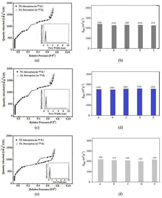
Figure 1. (a) N2 adsorption isotherm of compound 6, (b) BET surface area of compound 6, (c) N2 adsorption isotherm of compound 7, (d) BET surface area of compound 7, (e) N2 adsorption isotherm of compound 8, (f) BET surface area of compound 8 (A: Pure, B: after terazosine hydrochloride loading, C: after telmisartan loading, D: after glimpiride loading, E: after rosuvastatin loading)
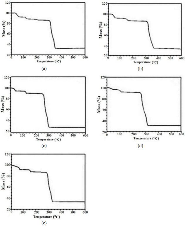
Figure 2. TGA plot of compound 6, (a) Pure, (b) after terazosine hydrochloride loading, (c) after telmisartan loading, (d) after glimpiride loading, (e) after rosuvastatin loading
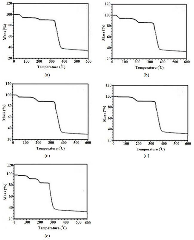
Figure 3. TGA plot of compound 7, (a) Pure, (b) after terazosine hydrochloride loading, (c) after telmisartan loading, (d) after glimpiride loading, (e) after rosuvastatin loading
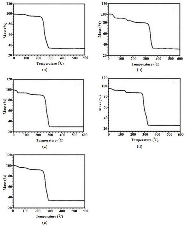
Figure 4. TGA plot of compound 8, (a) Pure, (b) after terazosine hydrochloride loading, (c) after telmisartan loading, (d) after glimpiride loading, (e) after rosuvastatin loading
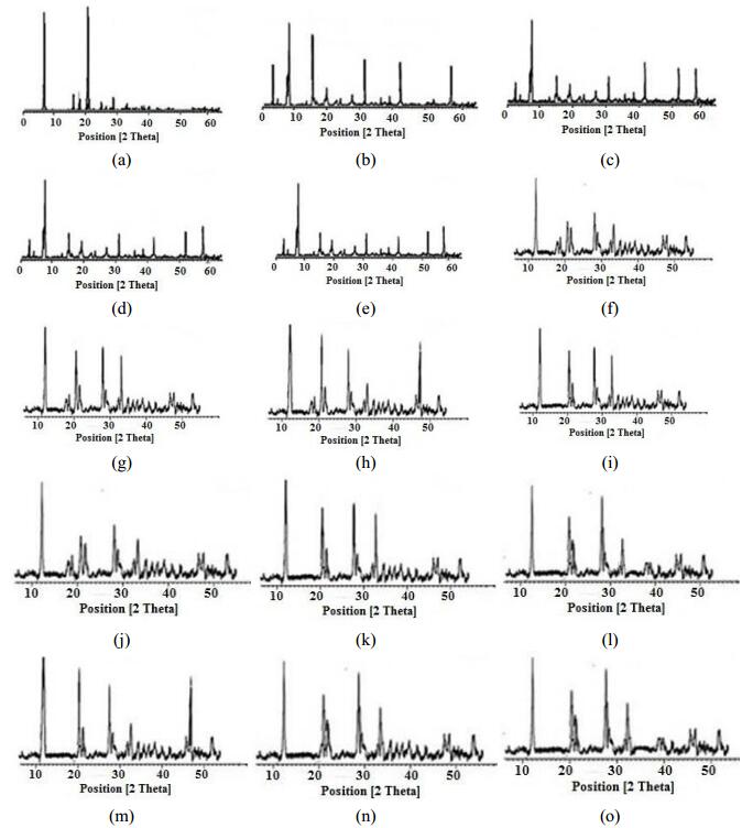
Figure 5. PXRD pattern of compound 6, (a) Pure, (b) after terazosine hydrochloride loading, (c) after telmisartan loading, (d) after glimpiride loading, (e) after rosuvastatin loading. PXRD pattern compound 7, (f) Pure, (g) after terazosine hydrochloride loading, (h) after telmisartan loading, (i) after glimpiride loading, (j) after rosuvastatin loading. PXRD pattern of compound 8, (k) Pure, (l) after terazosine hydrochloride loading, (m) after telmisartan loading, (n) after glimpiride loading, (o) after rosuvastatin loading


 DownLoad: