Uitdam, the Netherlands: test site for soft fibrous peat

C. Zwanenburg; G. Erkens; C. Zwanenburg; G. Erkens

doi:10.3934/geosci.2019.4.804

AIMS Geosciences

2019, Volume 5, Issue 4: 804-830. doi: 10.3934/geosci.2019.4.804

Previous Article Next Article

Research article Special Issues

Uitdam, the Netherlands: test site for soft fibrous peat

C. Zwanenburg ^{1
,
,},
G. Erkens ²

1.
Deltares, Delft, The Netherlands/Delft University of Technology, Delft, The Netherlands
2.
Deltares, Utrecht, The Netherlands/Utrecht University, Utrecht, The Netherlands

Received: 20 February 2019 Accepted: 09 August 2019 Published: 27 September 2019

Subsoil strata in the most densely populated areas of the Netherlands typically contain peat layers. Consequently, knowledge is required about the complex mechanical behaviour of peats for the purposes of the geotechnical design and maintenance of infrastructure. A test site was set up for a dike reinforcement project, primarily in order to determine the operational undrained shear strength of peats. The field trials, and extensive laboratory and field probe testing, showed that, although margins of uncertainty in the individual measurements are large, the combination of different testing techniques provides a clear image of the strength behaviour of peats. Additional testing of large samples showed the relevance of size effects for peat tests. The back analysis of the tests produced operational undrained shear strength values that concur closely with laboratory and field probe testing. These test results provide a direction for future research targeting the development of constitutive models to predict the stress—strain behaviour of peats correctly.

Keywords:

Citation: C. Zwanenburg, G. Erkens. Uitdam, the Netherlands: test site for soft fibrous peat[J]. AIMS Geosciences, 2019, 5(4): 804-830. doi: 10.3934/geosci.2019.4.804

Related Papers:

[1]	Mahmoud S. Mehany, Faizah D. Alanazi . An $\eta$ -Hermitian solution to a two-sided matrix equation and a system of matrix equations over the skew-field of quaternions. AIMS Mathematics, 2025, 10(4): 7684-7705. doi: 10.3934/math.2025352
[2]	Abdur Rehman, Muhammad Zia Ur Rahman, Asim Ghaffar, Carlos Martin-Barreiro, Cecilia Castro, Víctor Leiva, Xavier Cabezas . Systems of quaternionic linear matrix equations: solution, computation, algorithm, and applications. AIMS Mathematics, 2024, 9(10): 26371-26402. doi: 10.3934/math.20241284
[3]	Vladislav N. Kovalnogov, Ruslan V. Fedorov, Denis A. Demidov, Malyoshina A. Malyoshina, Theodore E. Simos, Spyridon D. Mourtas, Vasilios N. Katsikis . Computing quaternion matrix pseudoinverse with zeroing neural networks. AIMS Mathematics, 2023, 8(10): 22875-22895. doi: 10.3934/math.20231164
[4]	Wenxv Ding, Ying Li, Anli Wei, Zhihong Liu . Solving reduced biquaternion matrices equation $\sum\limits_{i = 1}^{k}A_iXB_i = C$ with special structure based on semi-tensor product of matrices. AIMS Mathematics, 2022, 7(3): 3258-3276. doi: 10.3934/math.2022181
[5]	Abdur Rehman, Cecilia Castro, Víctor Leiva, Muhammad Zia Ur Rahman, Carlos Martin-Barreiro . Solving two-sided Sylvester quaternionic matrix equations: Theoretical insights, computational implementation, and practical applications. AIMS Mathematics, 2025, 10(7): 15663-15697. doi: 10.3934/math.2025702
[6]	Yang Chen, Kezheng Zuo, Zhimei Fu . New characterizations of the generalized Moore-Penrose inverse of matrices. AIMS Mathematics, 2022, 7(3): 4359-4375. doi: 10.3934/math.2022242
[7]	Abdur Rehman, Ivan Kyrchei, Muhammad Zia Ur Rahman, Víctor Leiva, Cecilia Castro . Solvability and algorithm for Sylvester-type quaternion matrix equations with potential applications. AIMS Mathematics, 2024, 9(8): 19967-19996. doi: 10.3934/math.2024974
[8]	Anli Wei, Ying Li, Wenxv Ding, Jianli Zhao . Three special kinds of least squares solutions for the quaternion generalized Sylvester matrix equation. AIMS Mathematics, 2022, 7(4): 5029-5048. doi: 10.3934/math.2022280
[9]	Dong Wang, Ying Li, Wenxv Ding . The least squares Bisymmetric solution of quaternion matrix equation $AXB = C$ . AIMS Mathematics, 2021, 6(12): 13247-13257. doi: 10.3934/math.2021766
[10]	Qi Xiao, Jin Zhong . Characterizations and properties of hyper-dual Moore-Penrose generalized inverse. AIMS Mathematics, 2024, 9(12): 35125-35150. doi: 10.3934/math.20241670

Abstract

1. Introduction

In this paper, we establish the following four symmetric quaternion matrix systems:

$\begin{align} \begin{aligned} \left\{\begin{array}{c} A_{11}X_1 = B_{11}, C_{11}X_1D_{11} = E_{11},\\ X_2A_{22} = B_{22}, C_{22}X_2D_{22} = E_{22},\\ F_{11}X_1H_{11}+X_2F_{22} = G_{11}, \end{array} \right. \end{aligned} \end{align}$

(1.1)

$\begin{align} \begin{aligned} \left\{\begin{array}{c} A_{11}X_1 = B_{11}, C_{11}X_1D_{11} = E_{11},\\ X_2A_{22} = B_{22}, C_{22}X_2D_{22} = E_{22},\\ F_{11}X_1+H_{11}X_2F_{22} = G_{11}, \end{array} \right. \end{aligned} \end{align}$

(1.2)

$\begin{align} \begin{aligned} \left\{\begin{array}{c} A_{11}X_1 = B_{11}, C_{11}X_1D_{11} = E_{11},\\ A_{22}X_2 = B_{22}, C_{22}X_2D_{22} = E_{22},\\ F_{11}X_1+H_{11}X_2F_{22} = G_{11}, \end{array} \right. \end{aligned} \end{align}$

(1.3)

$\begin{align} \begin{aligned} \left\{\begin{array}{c} A_{11}X_1 = B_{11}, C_{11}X_1D_{11} = E_{11},\\ A_{22}X_2 = B_{22}, C_{22}X_2D_{22} = E_{22},\\ F_{11}X_1+X_2F_{22} = G_{11}, \end{array} \right. \end{aligned} \end{align}$

(1.4)

where $A_{ii}, \ B_{ii}, \ C_{ii}, \ D_{ii}, \ E_{ii}, \ F_{ii}(i = \overline{1, 2})$ , $H_{11}$ , and $G_{11}$ are known matrices, while $X_i (i = \overline{1, 2})$ are unknown.

In this paper, $\mathbb{R}$ and $\mathbb{H}^{m\times n}$ denote the real number field and the set of all quaternion matrices of order $m\times n$ , respectively.

$\begin{align*} &\mathbb{H} = \{v_{0}+v_{1}\mathbf{i}+v_{2}\mathbf{j}+v_{3}\mathbf{k} | \mathbf{i}^{2} = \mathbf{j}^{2} = \mathbf{k}^{2} = \mathbf{ijk} = -1, v_{0}, v_{1}, v_{2}, v_{3}\in \mathbb{R}\}. \end{align*}$

Moreover, $r(A)$ , $0$ and $I$ represent the rank of matrix $A$ , the zero matrix of suitable size, and the identity matrix of suitable size, respectively. The conjugate transpose of $A$ is $A^{\ast}$ . For any matrix $A$ , if there exists a unique solution $X$ such that

$\begin{align*} AXA = A, XAX = X, (AX)^{\ast} = AX, (XA)^{\ast} = XA, \end{align*}$

then $X$ is called the Moore-Penrose ( $M-P$ ) inverse. It should be noted that $A^{\dagger}$ is used to represent the $M-P$ inverse of $A$ . Additionally, $L_{A} = I-A^{\dagger}A$ and $R_{A} = I-AA^{\dagger}$ denote two projectors toward $A$ .

$\mathbb{H}$ is known to be an associative noncommutative division algebra over $\mathbb{R}$ with extensive applications in computer science, orbital mechanics, signal and color image processing, control theory, and so on (see ^[1,2,3,4]).

Matrix equations, significant in the domains of descriptor systems control theory ^[5], nerve networks ^[6], back feed ^[7], and graph theory ^[8], are one of the key research topics in mathematics.

The study of matrix equations in $\mathbb{H}$ has garnered the attention of various researchers; consequently they have been analyzed by many studies (see, e.g., ^[9,10,11,12]). Among these the system of symmetric matrix equations is a crucial research object. For instance, Mahmoud and Wang ^[13] established some necessary and sufficient conditions for the three symmetric matrix systems in terms of $M-P$ inverses and rank equalities:

$\begin{equation} \begin{aligned} \left\{\begin{array}{c} A_{1}V = C_1,\ VB_1 = C_2,\\ A_3X+YB_3 = C_3,\\ A_2Y+ZB_2+A_5VB_5 = C_5,\\ A_4W+ZB_4 = C_4,\\ \end{array} \right. \left\{\begin{array}{c} A_{1}V = C_1,\ VB_1 = C_2,\\ A_3X+YB_3 = C_3,\\ A_2Z+YB_2+A_5VB_5 = C_5,\\ A_4Z+WB_4 = C_4,\\ \end{array} \right. \left\{\begin{array}{c} A_{1}V = C_1,\ VB_1 = C_2,\\ A_3X+YB_3 = C_3,\\ A_2Y+ZB_2+A_5VB_5 = C_5,\\ A_4Z+WB_4 = C_4. \end{array} \right. \end{aligned} \end{equation}$

(1.5)

Wang and He ^[14] established the sufficient and necessary conditions for the existence of solutions to the following three symmetric coupled matrix equations and the expressions for their general solutions:

$\begin{equation} \begin{aligned} \left\{\begin{array}{c} A_{1}X+YB_1 = C_1,\\ A_2Y+ZB_2 = C_2,\\ A_3W+ZB_3 = C_3,\\ \end{array} \right. \left\{\begin{array}{c} A_{1}X+YB_1 = C_1,\\ A_2Z+YB_2 = C_2,\\ A_3Z+WB_3 = C_3,\\ \end{array} \right. \left\{\begin{array}{c} A_{1}X+YB_1 = C_1,\\ A_2Y+ZB_2 = C_2,\\ A_3Z+WB_3 = C_3. \\ \end{array} \right. \end{aligned} \end{equation}$

(1.6)

It is noteworthy that the following matrix equation plays an important role in the analysis of the solvability conditions of systems (1.1)–(1.4):

$\begin{equation} \begin{aligned} A_1U+VB_1+A_2XB_2+A_3YB_3+A_4ZB_4 = B. \end{aligned} \end{equation}$

(1.7)

Liu et al. ^[15] derived some necessary and sufficient conditions to solve the quaternion matrix equation (1.7) using the ranks of coefficient matrices and $M-P$ inverses. Wang et al. ^[16] derived the following quaternion equations after obtaining some solvability conditions for the quaternion equation presented in Eq (1.8) in terms of $M-P$ inverses:

$\begin{equation} \begin{aligned} \left\{\begin{array}{c} A_{11}X_1 = B_{11}, C_{11}X_1D_{11} = E_{11},\\ X_2A_{22} = B_{22}, C_{22}X_2D_{22} = E_{22},\\ F_{11}X_1+X_2F_{22} = G_{11}. \end{array} \right. \end{aligned} \end{equation}$

(1.8)

To our knowledge, so far, there has been little information on the solvability conditions and an expression of the general solution to systems (1.1)–(1.4).

In mathematical research and applications, the concept of $\eta$ -Hermitian matrices has gained significant attention ^[17]. An $\eta$ -Hermitian matrix, for $\eta \in \{\mathbf{i}, \mathbf{j}, \mathbf{k}\}$ , is defined as a matrix $A$ such that $A = A^{\eta^{*}}$ , where $A^{\eta^{*}} = -\eta A^{*}\eta$ . These matrices have found applications in various fields including linear modeling and the statistics of random signals ^[1,17]. As an application of (1.1), this paper establishes some necessary and sufficient conditions for the following matrix equation:

$\begin{equation} \begin{aligned} \left\{\begin{array}{c} A_{11}X_1 = B_{11}, C_{11}X_1C_{11}^{\eta^{*}} = E_{11},\\ F_{11}X_1F_{11}^{\eta^{*}}+(F_{22}X_1)^{\eta^{*}} = G_{11} \end{array} \right. \end{aligned} \end{equation}$

(1.9)

to be solvable.

Motivated by the study of Systems (1.8), symmetric matrix equations, $\eta$ -Hermitian matrices, and the widespread use of matrix equations and quaternions as well as the need for their theoretical advancements, we examine the solvability conditions of the quaternion systems presented in systems (1.1)–(1.4) by utilizing the rank equalities and the $M-P$ inverses of coefficient matrices. We then obtain the general solutions for the solvable quaternion equations in systems (1.1)–(1.4). As an application of (1.1), we utilize the $M-P$ inverse and the rank equality of matrices to investigate the necessary and sufficient conditions for the solvability of quaternion matrix equations involving $\eta$ -Hermicity matrices. It is evident that System (1.8) is a specific instance of System (1.1).

The remainder of this article is structured as follows. Section 2 outlines the basics. Section 3 examines some solvability conditions of the quaternion equation presented in System (1.1) using the $M-P$ inverses and rank equalities of the matrices, and derives the solution of System (1.1). Section 4 establishes some solvability conditions for matrix systems (1.2)–(1.4) to be solvable. Section 5 investigates some necessary and sufficient conditions for matrix equation (1.9) to have common solutions. Section 6 concludes the paper.

2. Preliminaries

Marsaglia and Styan ^[18] presented the following rank equality lemma over the complex field, which can be generalized to $\mathbb{H}$ .

Lemma 2.1. ^[18] Let $A \in \mathbb{H}^{m\times n}$ , $B \in \mathbb{H}^{m\times k}$ , $C \in \mathbb{H}^{l\times n}$ , $D \in \mathbb{H}^{j\times k},$ and $E \in \mathbb{H}^{l\times i}$ be given. Then, the following rank equality holds:

$\ r\begin{pmatrix} A&BL_{D}\\ R_{E}C&0 \end{pmatrix} = r\begin{pmatrix} A&B&0\\ C&0&E\\ 0&D&0 \end{pmatrix}-r\begin{pmatrix} D \end{pmatrix}-r\begin{pmatrix} E \end{pmatrix}.$

Lemma 2.2. ^[19] Let $A \in \mathbb{H}^{m\times n}$ be given. Then,

$\begin{align*} &(1)\quad (A^{\eta})^{\dagger} = (A^{\dagger})^{\eta}, (A^{\eta^{*}})^{\dagger} = (A^{\dagger})^{\eta^{*}};\\ & (2)\quad r(A) = r(A^{\eta^{*}}) = r(A^{\eta});\\ & (3)\quad (L_A)^{\eta^{*}} = -\eta(L_A)\eta = (L_A)^{\eta} = L_{A^{\eta^{*}}} = R_{A^{\eta^{*}}},\\ & (4)\quad (R_A)^{\eta^{*}} = -\eta(R_A)\eta = (R_A)^{\eta} = R_{A^{\eta^{*}}} = L_{A^{\eta^{*}}};\\ & (5)\quad (AA^{\dagger})^{\eta^{*}} = (A^{\dagger})^{\eta^{*}}A^{\eta^{*}} = (A^{\dagger}A)^{\eta} = A^{\eta}(A^{\dagger})^{\eta};\\ & (6)\quad (A^{\dagger}A)^{\eta^{*}} = A^{\eta^{*}}(A^{\dagger})^{\eta^{*}} = (AA^{\dagger})^{\eta} = (A^{\dagger})^{\eta}A^{\eta}. \end{align*}$

Lemma 2.3. ^[20] Let $A_{1}$ and $A_{2}$ be given quaternion matrices with adequate shapes. Then, the equation $A_{1}X = A_{2}$ is solvable if, and only if, $A_{2} = A_{1}A_{1}^{\dagger}A_{2}$ . In this case, the general solution to this equation can be expressed as

$X = A_{1}^{\dagger}A_{2}+L_{A_{1}}U_{1},$

where $U_{1}$ is any matrix with appropriate size.

Lemma 2.4. ^[20] Let $A_{1}$ and $A_{2}$ be given quaternion matrices with adequate shapes. Then, the equation $XA_{1} = A_{2}$ is solvable if, and only if, $A_{2} = A_{2}A_{1}^{\dagger}A_{1}$ . In this case, the general solution to this equation can be expressed as

$X = A_{2}A_{1}^{\dagger}+U_{1}R_{A_{1}},$

where $U_{1}$ is any matrix with appropriate size.

Lemma 2.5. ^[21] Let $A, B,$ and $C$ be known quaternion matrices with appropriate sizes. Then, the matrix equation

$\begin{align*} AXB = C \end{align*}$

is consistent if, and only if,

$\begin{align*} R_{A}C = 0,CL_{B} = 0. \end{align*}$

In this case, the general solution to this equation can be expressed as

$\begin{align*} X = A^{\dagger}CB^{\dagger}+L_{A}U+VR_{B}, \end{align*}$

where $U$ and $V$ are any quaternion matrices with appropriate sizes.

Lemma 2.6. ^[15] Let $C_{i}, D_{i}$ , and $Z \; (i = \overline{1, 4})$ be known quaternion matrices with appropriate sizes.

$\begin{equation} C_{1}X_{1}+X_{2}D_{1}+C_{2}Y_{1}D_{2}+C_{3}Y_{2}D_{3}+C_{4}Y_{3}D_{4} = Z. \end{equation}$

(2.1)

Denote

$\begin{align*} &R_{C_{1}}C_{2} = C_{12},R_{C_{1}}C_{3} = C_{13},R_{C_{1}}C_{4} = C_{14},D_{2}L_{D_{1}} = D_{21},D_{31}L_{D_{21}} = N_{32},D_{3}L_{D_{1}} = D_{31},\\ &D_{4}L_{D_{1}} = D_{41},R_{C_{12}}C_{13} = M_{23},S_{12} = C_{13}L_{M_{23}},R_{C_{1}}ZL_{D_{1}} = T_{1},C_{32} = R_{M_{23}}R_{C_{12}},A_{1} = C_{32}C_{14},\\ & A_{2} = R_{C_{12}}C_{14},A_{3} = R_{C_{13}}C_{14},A_{4} = C_{14},D_{13} = L_{D_{21}}L_{N_{32}},B_{1} = D_{41},B_{2} = D_{41}L_{D_{31}},\\ &B_{3} = D_{41}L_{D_{21}},B_{4} = D_{41}D_{13},E_{1} = C_{32}T_{1},E_{2} = R_{C_{12}}T_{1}L_{D_{31}},E_{3} = R_{C_{13}}T_{1}L_{D_{21}},E_{4} = T_{1}D_{13}, \\ &A_{24} = (L_{A_{2}},L_{A_{4}}),B_{13} = \begin{pmatrix} R_{B_{1}}\\R_{B_{3}} \end{pmatrix},A_{11} = L_{A_{1}},B_{22} = R_{B_{2}},A_{33} = L_{A_{3}},B_{44} = R_{B_{4}},E_{11} = R_{A_{24}}A_{11},\\ &E_{22} = R_{A_{24}}A_{33},E_{33} = B_{22}L_{B_{13}},E_{44} = B_{44}L_{B_{13}},N = R_{E_{11}}E_{22},M = E_{44}L_{E_{33}},K = K_{2}-K_{1},\\ &E = R_{A_{24}}KL_{B_{13}},S = E_{22}L_{N},K_{11} = A_{2}L_{A_{1}},G_{1} = E_{2}-A_{2}A_{1}^{\dagger}E_{1}B_{1}^{\dagger}B_{2},K_{22} = A_{4}L_{A_{3}},\\ &G_{2} = E_{4}-A_{4}A_{3}^{\dagger}E_{3}B_{3}^{\dagger}B_{4},K_{1} = A_{1}^{\dagger}E_{1}B_{1}^{\dagger}+L_{A_{1}}A_{2}^{\dagger}E_{2}B_{2}^{\dagger},K_{2} = A_{3}^{\dagger}E_{3}B_{3}^{\dagger}+L_{A_{3}}A_{4}^{\dagger}E_{4}B_{4}^{\dagger}. \end{align*}$

Then, the following statements are equivalent:

$\mathrm{(1)}$ Equation (2.1) is consistent.

$\mathrm{(2)}$

$\begin{align*} R_{A_{i}}E_{i} = 0,E_{i}L_{B_{i}} = 0(i = \overline{1,4}),R_{E_{11}}EL_{E_{44}} = 0. \end{align*}$

$\mathrm{(3)}$

$\begin{align*} \quad \quad \quad&r\begin{pmatrix} Z&C_{2}&C_{3}&C_{4}&C_{1}\\D_{1}&0&0&0&0 \end{pmatrix} = r(D_{1})+r(C_{2},C_{3},C_{4},C_{1}),\\ &r\begin{pmatrix} Z&C_{2}&C_{4}&C_{1}\\D_{3}&0&0&0\\D_{1}&0&0&0 \end{pmatrix} = r(C_{2},C_{4},C_{1})+r\begin{pmatrix} D_{3}\\D_{1} \end{pmatrix},\\ &r\begin{pmatrix} Z&C_{3}&C_{4}&C_{1}\\D_{2}&0&0&0\\D_{1}&0&0&0 \end{pmatrix} = r(C_{3},C_{4},C_{1})+r\begin{pmatrix} D_{2}\\D_{1} \end{pmatrix},\\ &r\begin{pmatrix} Z&C_{4}&C_{1}\\D_{2}&0&0\\D_{3}&0&0\\D_{1}&0&0 \end{pmatrix} = r\begin{pmatrix} D_{2}\\D_{3}\\D_{1} \end{pmatrix}+r(C_{4},C_{1}),\\ & r\begin{pmatrix} Z&C_{2}&C_{3}&C_{1}\\D_{4}&0&0&0\\D_{1}&0&0&0 \end{pmatrix} = r(C_{2},C_{3},C_{1})+r\begin{pmatrix} D_{4}\\D_{1} \end{pmatrix},\\ & r\begin{pmatrix} Z&C_{2}&C_{1}\\D_{3}&0&0\\D_{4}&0&0\\D_{1}&0&0 \end{pmatrix} = r\begin{pmatrix} D_{3}\\D_{4}\\D_{1} \end{pmatrix}+r(C_{2},C_{1}), \\ & r\begin{pmatrix} Z&C_{3}&C_{1}\\D_{2}&0&0\\D_{4}&0&0\\D_{1}&0&0 \end{pmatrix} = r\begin{pmatrix} D_{2}\\D_{4}\\D_{1} \end{pmatrix}+r(C_{3},C_{1}),\\\\ & r\begin{pmatrix} Z&C_{1}\\D_{2}&0\\D_{3}&0\\D_{4}&0\\D_{1}&0 \end{pmatrix} = r\begin{pmatrix} D_{2}\\D_{3}\\D_{4}\\D_{1} \end{pmatrix}+r(C_{1}),\\ &r\begin{pmatrix} Z&C_{2}&C_{1}&0&0&0&C_{4}\\D_{3}&0&0&0&0&0&0\\D_{1}&0&0&0&0&0&0\\0&0&0&-Z&C_{3}&C_{1}&C_{4}\\0&0&0&D_{2}&0&0&0\\0&0&0&D_{1}&0&0&0\\D_{4}&0&0&D_{4}&0&0&0 \end{pmatrix} = r\begin{pmatrix} D_{3}&0\\D_{1}&0\\0&D_{2}\\0&D_{1}\\D_{4}&D_{4} \end{pmatrix}+r\begin{pmatrix} C_{2}&C_{1}&0&0&C_{4}\\0&0&C_{3}&C_{1}&C_{4} \end{pmatrix}. \end{align*}$

Under these conditions, the general solution to the matrix equation (2.1) is

$\begin{align*} &X_{1} = C_{1}^{\dagger}(Z-C_{2}Y_{1}D_{2}-C_{3}Y_{2}D_{3}-C_{4}Y_{3}D_{4})-C_{1}^{\dagger}U_{1}D_{1}+L_{C_{1}}U_{2},\\ &X_{2} = R_{C_{1}}(Z-C_{2}Y_{1}D_{2}-C_{3}Y_{2}D_{3}-C_{4}Y_{3}D_{4})D_{1}^{\dagger}+C_{1}C_{1}^{\dagger}U_{1}+U_{3}R_{D_{1}},\\ &Y_{1} = C_{12}^{\dagger}TD_{21}^{\dagger}-C_{12}^{\dagger}C_{13}M_{23}^{\dagger}TD_{21}^{\dagger}-C_{12}^{\dagger}S_{12}C_{13}^{\dagger}TN_{32}^{\dagger}D_{31}D_{21}^{\dagger}\\ &\quad\quad-C_{12}^{\dagger}S_{12}U_{4}R_{N_{32}}D_{31}D_{21}^{\dagger}+L_{C_{12}}U_{5}+U_{6}R_{D_{21}},\\ &Y_{2} = M_{23}^{\dagger}TD_{31}^{\dagger}+S_{12}^{\dagger}S_{12}C_{13}^{\dagger}TN_{32}^{\dagger}+L_{M_{23}}L_{S_{12}}U_{7}+U_{8}R_{D_{31}}+L_{M_{23}}U_{4}R_{N_{32}},\\ &Y_{3} = K_{1}+L_{A_{2}}V_{1}+V_{2}R_{B_{1}}+L_{A_{1}}V_{3}R_{B_{2}},\ or\ Y_{3} = K_{2}-L_{A_{4}}W_{1}-W_{2}R_{B_{3}}-L_{A_{3}}W_{3}R_{B_{4}}, \end{align*}$

where $T = T_{1}-C_{4}Y_{3}D_{4}, U_{i}(i = \overline{1, 8})$ are arbitrary matrices with appropriate sizes over $\mathbb{H}$ ,

$\begin{align*} &V_{1} = (I_{m},0)[A_{24}^{\dagger}(K-A_{11}V_{3}B_{22}-A_{33}W_{3}B_{44})-A_{24}^{\dagger}U_{11}B_{13}+L_{A_{24}}U_{12}],\\ &W_{1} = (0,I_{m})[A_{24}^{\dagger}(K-A_{11}V_{3}B_{22}-A_{33}W_{3}B_{44})-A_{24}^{\dagger}U_{11}B_{13}+L_{A_{24}}U_{12}],\\ &W_{2} = [R_{A_{24}}(K-A_{11}V_{3}B_{22}-A_{33}W_{3}B_{44})B_{13}^{\dagger}+A_{24}A_{24}^{\dagger}U_{11}+U_{21}R_{B_{13}}]\begin{pmatrix} 0\\I_{n} \end{pmatrix},\\ &V_{2} = [R_{A_{24}}(K-A_{11}V_{3}B_{22}-A_{33}W_{3}B_{44})B_{13}^{\dagger}+A_{24}A_{24}^{\dagger}U_{11}+U_{21}R_{B_{13}}]\begin{pmatrix} I_{n}\\0 \end{pmatrix},\quad\quad\quad\quad\\ &V_{3} = E_{11}^{\dagger}KE_{33}^{\dagger}-E_{11}^{\dagger}E_{22}N^{\dagger}KE_{33}^{\dagger}-E_{11}^{\dagger}SE_{22}^{\dagger}KM^{\dagger}E_{44}E_{33}^{\dagger}\\ &\quad\quad-E_{11}^{\dagger}SU_{31}R_{M}E_{44}E_{33}^{\dagger}+L_{E_{11}}U_{32}+U_{33}R_{E_{33}},\quad\quad\quad\quad\quad\quad\quad\quad\quad\quad\quad\quad\quad\quad\quad\quad\\ &W_{3} = N^{\dagger}KE_{44}+S^{\dagger}SE_{22}^{\dagger}KM^{\dagger}+L_{N}L_{S}U_{41}+L_{N}U_{31}R_{M}-U_{42}R_{E_{44}}, \end{align*}$

$U_{11}, U_{12}, U_{21}, U_{31}, U_{32}, U_{33}, U_{41},$ and $U_{42}$ are arbitrary quaternion matrices with appropriate sizes, and $m$ and $n$ denote the column number of $C_{4}$ and the row number of $D_{4}$ , respectively.

3. Solvability conditions and expression of general solution for system (1.1)

Some necessary and sufficient conditions for System (1.1) to be solvable will be established in this section. The general solution of System (1.1) will also be derived in this section. Moreover, we provide an example to illustrate our main results.

Theorem 3.1. Let $A_{ii}, B_{ii}, C_{ii}, D_{ii}, E_{ii}, F_{ii}, H_{11},$ and $G_{11}$ (i = 1, 2) be given quaternion matrices. Put

$\begin{align} &\begin{aligned} \left\{\begin{array}{c} A_{1} = C_{11}L_{A_{11}},P_{1} = E_{11}-C_{11}A_{11}^{\dagger}B_{11}D_{11},B_{2} = R_{A_{22}}D_{22},\\ P_{2} = E_{22}-C_{22}B_{22}A_{22}^{\dagger}D_{22},\hat{B_{1}} = R_{B_{2}}R_{A_{22}}F_{22},\hat{A_{2}} = F_{11}L_{A_{11}}L_{A_{1}},\\ \hat{A_{3}} = {F_{11}}L_{A_{11}},\hat{B_{3}} = R_{D_{11}}H_{11},\hat{A_{4}} = L_{C_{22}},\hat{B_{4}} = R_{A_{22}}F_{22},H_{11}L_{\hat{B_{1}}} = \hat{B_{11}},\\ P = G_{11}-F_{11}A_{11}^{\dagger}B_{11}H_{11}-F_{11}L_{A_{11}}A_{1}^{\dagger}P_{1}D_{11}^{\dagger}H_{11}-B_{22}A_{22}^{\dagger}F_{22}-C_{22}^{\dagger}P_{2}B_{2}^{\dagger}R_{A_{22}}F_{22}, \end{array} \right. \end{aligned} \end{align}$

(3.1)

$\begin{align} &\begin{aligned} \left\{\begin{array}{c} \hat{B_{22}}L_{\hat{B_{11}}} = N_{1},\hat{B_{3}}L_{\hat{B_{1}}} = \hat{B_{22}},\hat{B_{4}}L_{\hat{B_{1}}} = \hat{B_{33}},R_{\hat{A_{2}}}\hat{A_{3}} = \hat{M_{1}},S_{1} = \hat{A_{3}}L_{\hat{M_{1}}}, T_1 = PL_{\hat{B_{1}}},\\ C = R_{\hat{M_{1}}}R_{\hat{A_{2}}},C_{1} = C\hat{A_{4}},C_{2} = R_{\hat{A_{2}}}\hat{A_{4}},C_{3} = R_{\hat{A_{3}}}\hat{A_{4}},C_{4} = \hat{A_{4}},D = L_{\hat{B_{11}}}L_{N_{1}},\\ D_{1} = \hat{B_{33}},D_{2} = \hat{B_{33}}L_{\hat{B_{22}}},D_{4} = \hat{B_{33}}D,E_{1} = CT_{1},E_{2} = R_{\hat{A_{2}}}T_{1}L_{\hat{B_{22}}}, \\ E_{3} = R_{\hat{A_{3}}}T_{1}L_{\hat{B_{11}}}, E_{4} = T_{1}D, \hat{C_{11}} = ( L_{C_{2}},L_{C_{4}}),D_{3} = \hat{B_{33}}L_{\hat{B_{11}}},\hat{D_{11}} = \begin{pmatrix} R_{D_{1}}\\ R_{D_{3}} \end{pmatrix},\\ \hat{C_{22}} = L_{C_{1}},\hat{D_{22}} = R_{D_{2}},\hat{C_{33}} = L_{C_{3}},\hat{D_{33}} = R_{D_{4}},\hat{E_{11}} = R_{\hat{C_{11}}}\hat{C_{22}},\\ \hat{E_{22}} = R_{\hat{C_{11}}}\hat{C_{22}},\hat{E_{33}} = \hat{D_{22}}L_{\hat{D_{11}}},\hat{E_{44}} = \hat{D_{33}}L_{\hat{D_{11}}},M = R_{\hat{E_{11}}}\hat{E_{22}},\\ N = \hat{E_{44}}L_{\hat{E_{33}}},F = F_{2}-F_{1},E = R_{\hat{C_{11}}}FL_{\hat{D_{11}}},S = \hat{E_{22}}L_{M},\hat{F_{11}} = C_{2}L_{C_{1}},\\ G_{1} = E_{2}-C_{2}C_{1}^{\dagger}E_{1}D_{1}^{\dagger}D_{2},\hat{F_{22}} = C_{4}L_{C_{3}},G_{2} = E_{4}-C_{4}C_{3}^{\dagger}E_{3}D_{3}^{\dagger}D_{4},\\ F_{1} = C_{1}^{\dagger}E_{1}D_{1}^{\dagger}+L_{C_{1}}C_{2}^{\dagger}E_{2}D_{2}^{\dagger},F_{2} = C_{3}^{\dagger}E_{3}D_{3}^{\dagger}+L_{C_{3}}C_{4}^{\dagger}E_{4}D_{4}^{\dagger}. \end{array} \right. \end{aligned} \end{align}$

(3.2)

Then, the following statements are equivalent:

$\mathrm{(1)}$ System (1.1) is solvable.

$\mathrm{(2)}$

$\begin{align*} &R_{A_{11}}B_{11} = 0,R_{A_{1}}P_{1} = 0,P_{1}L_{D_{11}} = 0,B_{22}L_{A_{22}} = 0,R_{C_{22}}P_{2} = 0,\\ &P_{2}L_{B_{2}} = 0,R_{C_{i}}E_{i} = 0,E_{i}L_{D_{i}} = 0(i = \overline{1,4}),R_{\hat{E_{11}}}EL_{\hat{E_{44}}} = 0. \end{align*}$

$\mathrm{(3)}$

$\begin{align} &\begin{aligned} &r(B_{11},A_{11}) = r(A_{11}), r\begin{pmatrix} E_{11}&C_{11}\\ B_{11}D_{11}&A_{11} \end{pmatrix} = r\begin{pmatrix} C_{11}\\A_{11} \end{pmatrix}, \end{aligned} \end{align}$

(3.3)

$\begin{align} &\begin{aligned} &r\begin{pmatrix} E_{11}\\D_{11} \end{pmatrix} = r(D_{11}), r\begin{pmatrix} B_{22}\\A_{22} \end{pmatrix} = r(A_{22}), \end{aligned} \end{align}$

(3.4)

$\begin{align} &\begin{aligned} & r(E_{22},C_{22}) = r(C_{22}), r\begin{pmatrix} E_{22}&C_{22}B_{22}\\D_{22}&A_{22} \end{pmatrix} = r(D_{22},A_{22}), \end{aligned} \end{align}$

(3.5)

$\begin{align} &\begin{aligned} & r\begin{pmatrix} F_{22}&0&D_{22}&A_{22}\\B_{11}H_{11}&A_{11}&0&0\\C_{22}G_{11}&C_{22}F_{11}&E_{22}&C_{22}B_{22} \end{pmatrix} = r(F_{22},D_{22},A_{22})+r\begin{pmatrix} A_{11}\\C_{22}F_{11} \end{pmatrix}, \end{aligned}\quad\quad\quad \end{align}$

(3.6)

$\begin{align} &\begin{aligned} & r\begin{pmatrix} H_{11}&0&-D_{11}&0&0\\ F_{22}&0&0&D_{22}&A_{22}\\ 0&C_{11}&E_{11}&0&0\\ 0&A_{11}&B_{11}D_{11}&0&0\\C_{22}G_{11}&C_{22}F_{11}&0&E_{22}&C_{22}B_{22} \end{pmatrix} \\ & = r\begin{pmatrix} C_{11}\\A_{11}\\C_{22}F_{11} \end{pmatrix}+r\begin{pmatrix} H_{11}&D_{11}&0&0\\F_{22}&0&D_{22}&A_{22} \end{pmatrix}, \end{aligned} \end{align}$

(3.7)

$\begin{align} &\begin{aligned} & r\begin{pmatrix} H_{11}&0&0&0\\ F_{22}&0&D_{22}&A_{22}\\0&A_{11}&0&0\\ C_{22}G_{11}&C_{22}F_{11}&E_{22}&C_{22}B_{22} \end{pmatrix} = r\begin{pmatrix} H_{11}&0&0\\F_{22}&D_{22}&A_{22} \end{pmatrix}+r\begin{pmatrix} A_{11}\\C_{22}F_{11} \end{pmatrix}, \end{aligned} \end{align}$

(3.8)

$\begin{align} &\begin{aligned} & r\begin{pmatrix} H_{11}&0&0\\F_{22}&D_{22}&A_{22}\\C_{22}G_{11}&E_{22}&C_{22}B_{22} \end{pmatrix} = r\begin{pmatrix} H_{11}&0&0\\F_{22}&D_{22}&A_{22} \end{pmatrix}, \end{aligned} \end{align}$

(3.9)

$\begin{align} &\begin{aligned} & r\begin{pmatrix} G_{11}&F_{11}&B_{22}\\F_{22}&0&A_{22}\\B_{11}H_{11}&A_{11}&0 \end{pmatrix} = r\begin{pmatrix} F_{11}\\A_{11} \end{pmatrix}+r(F_{22},A_{22}), \end{aligned} \end{align}$

(3.10)

$\begin{align} &\begin{aligned} & r\begin{pmatrix} G_{11}&F_{11}&0&B_{22}\\H_{11}&0&-D_{11}&0\\F_{22}&0&0&A_{22}\\0&C_{11}&E_{11}&0\\0&A_{11}&B_{11}D_{11}&0 \end{pmatrix} = r\begin{pmatrix} H_{11}&D_{11}&0\\F_{22}&0&A_{22} \end{pmatrix}+r\begin{pmatrix} F_{11}\\C_{11}\\A_{11} \end{pmatrix}, \end{aligned} \end{align}$

(3.11)

$\begin{align} &\begin{aligned} & r\begin{pmatrix} G_{11}&F_{11}&B_{22}\\H_{11}&0&0\\F_{22}&0&A_{22}\\0&A_{11}&0 \end{pmatrix} = r\begin{pmatrix} H_{11}&0\\F_{22}&A_{22} \end{pmatrix}+r\begin{pmatrix} F_{11}\\A_{11} \end{pmatrix}, \end{aligned} \end{align}$

(3.12)

$\begin{align} &\begin{aligned} & r\begin{pmatrix} G_{11}&B_{22}\\H_{11}&0\\F_{22}&A_{22} \end{pmatrix} = r\begin{pmatrix} H_{11}&0\\F_{22}&A_{22} \end{pmatrix},\end{aligned} \end{align}$

(3.13)

$\begin{align} &\begin{aligned} &r\begin{pmatrix} H_{11}&0&0&0&0&0&0&D_{11}&0\\F_{22}&0&0&0&0&D_{22}&A_{22}&0&0\\0&0&H_{11}&0&0&0&0&0&0\\0&0&F_{22}&D_{22}&A_{22}&0&0&0&0\\F_{22}&0&F_{22}&0&0&0&0&0&A_{22}\\ 0&C_{11}&0&0&0&0&0&-E_{11}&0\\0&A_{11}&0&0&0&0&0&-B_{11}D_{11}&0\\C_{22}G_{11}&C_{22}F_{11}&0&0&0&E_{22}&C_{22}B_{22}&0&0 \end{pmatrix}\\ & = r\left(\begin{array}{cccccccc} H_{11} & 0 & 0 & 0 & 0 & 0 & D_{11} & 0 \\ F_{22} & 0 & 0 & 0 & D_{22} & A_{22} & 0 & 0 \\ 0 & H_{11} & 0 & 0 & 0 & 0 & 0 & 0 \\ 0 & F_{22} & D_{22} & A_{22} & 0 & 0 & 0 & 0 \\ F_{22} & F_{22} & 0 & 0 & 0 & 0 & 0 & A_{22} \end{array}\right)+r\left(\begin{array}{c} C_{11} \\ A_{11} \\ C_{22} F_{11} \end{array}\right). \end{aligned} \end{align}$

(3.14)

Proof. $(1)\Leftrightarrow (2)$ : The System (1.1) can be written as follows.

$\begin{align} \begin{aligned} A_{11}X_1 = B_{11},\ X_{2}A_{22} = B_{22},\quad\quad \end{aligned} \end{align}$

(3.15)

$\begin{align} \begin{aligned} C_{11}X_1D_{11} = E_{11},\ C_{22}X_2D_{22} = E_{22}, \end{aligned} \end{align}$

(3.16)

and

$\begin{align} F_{11}X_1H_{11}+X_2F_{22} = G_{11}. \end{align}$

(3.17)

Next, the solvability conditions and the expression for the general solutions of Eq (3.15) to Eq (3.17) are given by the following steps:

Step 1: According to Lemma 2.3 and Lemma 2.4, the system (3.15) is solvable if, and only if,

$\begin{align} R_{A_{11}}B_{11} = 0,\ B_{22}L_{A_{22}} = 0. \end{align}$

(3.18)

When condition (3.18) holds, the general solution of System (3.15) is

$\begin{align} X_1 = A_{11}^{\dagger}B_{11}+L_{A_{11}}U_1,\ X_2 = B_{22}A_{22}^{\dagger}+U_2R_{A_{22}}. \end{align}$

(3.19)

Step 2: Substituting (3.19) into (3.16) yields,

$\begin{align} A_{1}U_{1}D_{11} = P_{1},\ C_{22}U_2B_{2} = P_{2}, \end{align}$

(3.20)

where $A_{1}, P_1, B_{2}, P_{2}$ are defined by (3.1). By Lemma 2.5, the system (3.20) is consistent if, and only if,

$\begin{align} R_{A_{1}}P_{1} = 0,\ P_{1}L_{D_{11}} = 0,\ R_{C_{22}}P_{2} = 0,\ P_{2}L_{B_{2}} = 0. \end{align}$

(3.21)

When (3.21) holds, the general solution to System (3.20) is

$\begin{align} U_{1} = A_{1}^{\dagger}P_{1}D_{11}^{\dagger}+L_{A_{1}}W_{1}+W_{2}R_{D_{11}}, U_2 = C_{22}^{\dagger}P_{2}B_{2}^{\dagger}+L_{C_{22}}W_{3}+W_{4}R_{B_{2}}. \end{align}$

(3.22)

Comparing (3.22) and (3.19), hence,

$\begin{align} \begin{aligned} X_{1} = A_{11}^{\dagger}B_{11}+L_{A_{11}}A_{1}^{\dagger}P_{1}D_{11}^{\dagger}+L_{A_{11}}L_{A_{1}}W_{1}+L_{A_{11}}W_{2}R_{D_{11}},\\ X_{2} = B_{22}A_{22}^{\dagger}+C_{22}^{\dagger}P_{2}B_{2}^{\dagger}R_{A_ {22}}+L_{C_{22}}W_{3}R_{A_{22}}+W_{4}R_{B_{2}}R_{A_{22}}. \end{aligned} \end{align}$

(3.23)

Step 3: Substituting (3.23) into (3.17) yields

$\begin{align} W_{4}\hat{B_{1}}+\hat{A_{2}}W_{1}H_{11}+\hat{A_{3}}W_{2}\hat{B_{3}}+\hat{A_{4}}W_{3}\hat{B_{4}} = P, \end{align}$

(3.24)

where $\hat{B_{i}}, \hat{A_{j}}(i = \overline{1, 4}, j = \overline{2, 4})$ are defined by (3.1). It follows from Lemma 2.6 that Eq (3.24) is solvable if, and only if,

$\begin{align} R_{C_{i}}E_{i} = 0, E_{i}L_{D_{i}} = 0(i = \overline{1,4}),R_{\hat{E_{11}}}EL_{\hat{E_{44}}} = 0. \end{align}$

(3.25)

When (3.25) holds, the general solution to matrix equation (3.24) is

where $C_{i}, E_{i}, D_{i}(i = \overline{1, 4}), \hat{E_{11}}, \hat{E_{44}}$ are defined as (3.2), $T = T_{1}-\hat{A_{4}}W_{3}\hat{B_{4}}, V_{i}(i = \overline{1, 8})$ are arbitrary matrices with appropriate sizes over $\mathbb{H}$ ,

$\begin{align*} &\hat{V_{1}} = (I_{m},0)[\hat{C_{11}}^{\dagger}(F-\hat{C_{22}}V_{3}\hat{D_{22}}-\hat{C_{33}}\hat{V_{3}}\hat{D_{33}})-\hat{C_{11}}^{\dagger}U_{11}\hat{D_{11}}+L_{\hat{C_{11}}}U_{12}],\\ &V_{1} = (0,I_{m})[\hat{C_{11}}^{\dagger}(F-\hat{C_{22}}V_{3}\hat{D_{22}}-\hat{C_{33}}\hat{V_{3}}\hat{D_{33}})-\hat{C_{11}}^{\dagger}U_{11}\hat{D_{11}}+L_{\hat{C_{11}}}U_{12}],\\ &V_{2} = [R_{\hat{C_{11}}}(F-\hat{C_{22}}V_{3}\hat{D_{22}}-\hat{C_{33}}\hat{V_{3}}\hat{D_{33}})\hat{D_{11}}^{\dagger}+\hat{C_{11}}\hat{C_{11}}^{\dagger}U_{11}+U_{21}R_{\hat{D_{11}}}]\begin{pmatrix} 0 \\ I_{n} \end{pmatrix},\\ &\hat{V_{2}} = [R_{\hat{C_{11}}}(F-\hat{C_{22}}V_{3}\hat{D_{22}}-\hat{C_{33}}\hat{V_{3}}\hat{D_{33}})\hat{D_{11}}^{\dagger}+\hat{C_{11}}\hat{C_{11}}^{\dagger}U_{11}+U_{21}R_{\hat{D_{11}}}]\begin{pmatrix} I_{n} \\ 0 \end{pmatrix},\\ &\hat{V_{3}} = \hat{E_{11}}^{\dagger}F\hat{E_{33}}^{\dagger}-\hat{E_{11}}^{\dagger}\hat{E_{22}}M^{\dagger}F\hat{E_{33}}^{\dagger}-\hat{E_{11}}^{\dagger}S\hat{E_{22}}^{\dagger}FN^{\dagger}\hat{E_{44}}\hat{E_{33}}^{\dagger}-\hat{E_{11}}^{\dagger}SU_{31}R_{N}\hat{E_{44}}\hat{E_{33}}^{\dagger}\\ &\quad\quad+L_{\hat{E_{11}}}U_{32}+U_{33}R_{\hat{E_{33}}},\\ &V_{3} = M^{\dagger}F\hat{E_{44}}^{\dagger}+S^{\dagger}S\hat{E_{22}}^{\dagger}FN^{\dagger}+L_{M}L_{S}U_{41}+L_{M}U_{31}R_{N}-U_{42}R_{\hat{E_{44}}}, \end{align*}$

$U_{11}, U_{12}, U_{21}, U_{31}, U_{32}, U_{33}, U_{41},$ and $U_{42}$ are any quaternion matrices with appropriate sizes, and $m$ and $n$ denote the column number of $C_{22}$ and the row number of $A_{22}$ , respectively. We summarize that System (1.1) has a solution if, and only if, (3.18), (3.21), and (3.25) hold, i.e., the System (1.1) has a solution if, and only if, (2) holds.

$(2)\Leftrightarrow (3)$ : We prove the equivalence in two parts. In the first part, we want to show that (3.18) and (3.21) are equivalent to (3.3) to (3.5), respectively. In the second part, we want to show that (3.25) is equivalent to (3.6) to (3.14). It is easy to know that there exist $X_{1}^{0}, X_{2}^{0}, U_{1}^{0},$ and $U_{2}^{0}$ such that

$\begin{align*} &A_{11}X_{1}^{0} = B_{11},\ X_{2}^{0}A_{22} = B_{22},\\ &A_1U_{1}^{0}D_{11} = P_{1},\ C_{22}U_{2}^{0}B_{2} = P_{2} \end{align*}$

holds, where

$\begin{align*} &X_{1}^{0} = A_{11}^{\dagger}B_{11}, U_{1}^{0} = A_{1}^{\dagger}P_{1}D_{11}^{\dagger},\\ &X_{2}^{0} = B_{22}A_{22}^{\dagger}, U_{2}^{0} = C_{22}^{\dagger}P_{2}B_{2}^{\dagger}, \end{align*}$

$P_{1} = E_{11}-C_{11}X_{1}^{0}D_{11}, P_{2} = E_{22}-C_{22}X_{2}^{0}D_{22},$ and $P = G_{11}-F_{11}X_{1}^{0}H_{11}-F_{11}L_{A_{11}}U_{1}^{0}H_{11}-X_{2}^{0}F_{22}-U_{2}^{0}R_{A_{22}}F_{22}.$

Part 1: We want to show that (3.18) and (3.21) are equivalent to (3.3) to (3.5), respectively. It follows from Lemma 2.1 and elementary transformations that

$\begin{align*} &(3.18) \Leftrightarrow r(R_{A_{11}}B_{11}) = 0 \Leftrightarrow r(B_{11},A_{11}) = r(A_{11}) \Leftrightarrow (3.3),\\ &(3.21) \Leftrightarrow r(R_{A_{1}}P_{1}) = 0 \Leftrightarrow r(P_{1},A_{1}) = r(A_{1}) \Leftrightarrow r(E_{11}-C_{11}A_{11}^{\dagger}B_{11}D_{11},C_{11}L_{A_{11}})\\ &\quad\quad\quad\quad = r(C_{11}L_{A_{11}}) \Leftrightarrow r\begin{pmatrix} E_{11}&C_{11}\\B_{11}D_{11}&A_{11} \end{pmatrix} = r\begin{pmatrix} C_{11}\\A_{11} \end{pmatrix} \Leftrightarrow (3.3),\\ &(3.21) \Leftrightarrow r(P_{1}L_{D_{11}}) = 0 \Leftrightarrow r\begin{pmatrix} P_{1}\\D_{11} \end{pmatrix} = r(D_{11}) \Leftrightarrow r\begin{pmatrix} E_{11}-C_{11}A_{11}^{\dagger}B_{11}D_{11}\\D_{11} \end{pmatrix}\\ &\quad\quad\quad\quad = r(D_{11}) \Leftrightarrow r\begin{pmatrix} E_{11}\\D_{11} \end{pmatrix} = r(D_{11}) \Leftrightarrow (3.4),\\ &(3.18) \Leftrightarrow r(B_{22}L_{A_{22}}) = 0 \Leftrightarrow r\begin{pmatrix} B_{22}\\A_{22} \end{pmatrix} = r(A_{22}) \Leftrightarrow (3.4).\quad \quad \quad \quad\quad \quad\quad\quad\quad \end{align*}$

Similarly, we can show that (3.21) is equivalent to (3.5). Hence, (3.18) and (3.21) are equivalent to (3.3) and (3.5), respectively.

Part 2: In this part, we want to show that (3.25) is equivalent to (3.6) and (3.14). According to Lemma 2.6, we have that (3.25) is equivalent to the following:

$\begin{align} &\begin{aligned} r\begin{pmatrix} P&\hat{A_{2}}&\hat{A_{3}}&\hat{A_{4}}\\ \hat{B_{1}}&0&0&0 \end{pmatrix} = r(\hat{B_{1}})+r(\hat{A_{2}},\hat{A_{3}},\hat{A_{4}}),\quad\quad\quad\quad\quad\quad\quad\quad\quad\quad \end{aligned} \end{align}$

(3.26)

$\begin{align} &\begin{aligned} r\begin{pmatrix} P&\hat{A_{2}}&\hat{A_{4}}\\\hat{B_{3}}&0&0\\\hat{B_{1}}&0&0 \end{pmatrix} = r(\hat{A_{2}},\hat{A_{4}})+r\begin{pmatrix} \hat{B_{3}}\\\hat{B_{1}} \end{pmatrix}, \end{aligned} \end{align}$

(3.27)

$\begin{align} &\begin{aligned} r\begin{pmatrix} P&\hat{A_{3}}&\hat{A_{4}}\\H_{11}&0&0\\\hat{B_{1}}&0&0 \end{pmatrix} = r(\hat{A_{3}},\hat{A_{4}})+r\begin{pmatrix} H_{11}\\\hat{B_{1}} \end{pmatrix}, \end{aligned} \end{align}$

(3.28)

$\begin{align} &\begin{aligned} r\begin{pmatrix} P&\hat{A_{4}}\\H_{11}&0\\\hat{B_{3}}&0\\\hat{B_{1}}&0 \end{pmatrix} = r\begin{pmatrix} H_{11}\\\hat{B_{3}}\\\hat{B_{1}} \end{pmatrix}+r(\hat{A_{4}}), \end{aligned} \end{align}$

(3.29)

$\begin{align} &\begin{aligned} r\begin{pmatrix} P&\hat{A_{2}}&\hat{A_{3}}\\\hat{B_{4}}&0&0\\\hat{B_{1}}&0&0 \end{pmatrix} = r(\hat{A_{2}},\hat{A_{3}})+r\begin{pmatrix} \hat{B_{4}}\\\hat{B_{1}} \end{pmatrix}, \end{aligned} \end{align}$

(3.30)

$\begin{align} &\begin{aligned} r\begin{pmatrix} P&\hat{A_{2}}\\\hat{B_{3}}&0\\\hat{B_{4}}&0\\\hat{B_{1}}&0 \end{pmatrix} = r\begin{pmatrix} \hat{B_{3}}\\\hat{B_{4}}\\\hat{B_{1}} \end{pmatrix}+r(\hat{A_{2}}), \end{aligned} \end{align}$

(3.31)

$\begin{align} &\begin{aligned} r\begin{pmatrix} P&\hat{A_{3}}\\H_{11}&0\\\hat{B_{4}}&0\\\hat{B_{1}}&0 \end{pmatrix} = r\begin{pmatrix} H_{11}\\\hat{B_{4}}\\\hat{B_{1}} \end{pmatrix}+r(\hat{A_{3}}), \end{aligned} \end{align}$

(3.32)

$\begin{align} &\begin{aligned} r\begin{pmatrix} P\\H_{11}\\\hat{B_{3}}\\\hat{B_{4}}\\\hat{B_{1}} \end{pmatrix} = r\begin{pmatrix} H_{11}\\\hat{B_{3}}\\\hat{B_{4}}\\\hat{B_{1}} \end{pmatrix}, \end{aligned} \end{align}$

(3.33)

$\begin{align} &\begin{aligned} &r\begin{pmatrix} P&\hat{A_{2}}&0&0&\hat{A_{4}}\\\hat{B_{3}}&0&0&0&0\\\hat{B_{1}}&0&0&0&0\\0&0&-P&\hat{A_{3}}&\hat{A_{4}}\\0&0&H_{11}&0&0\\0&0&\hat{B_{1}}&0&0\\\hat{B_{4}}&0&\hat{B_{4}}&0&0 \end{pmatrix} \end{aligned} = r\begin{pmatrix} \hat{B_{3}}&0\\\hat{B_{1}}&0\\0&H_{11}\\0&\hat{B_{1}}\\\hat{B_{4}}&\hat{B_{4}} \end{pmatrix}+r\begin{pmatrix} \hat{A_{2}}&0&\hat{A_{4}}\\0&\hat{A_{3}}&\hat{A_{4}} \end{pmatrix}, \end{align}$

(3.34)

respectively. Hence, we only prove that (3.26)–(3.34) are equivalent to (3.6)–(3.14) when we prove that (3.25) is equivalent to (3.6)–(3.14). Now, we prove that (3.26)–(3.34) are equivalent to (3.6)–(3.14). In fact, we only prove that (3.26), (3.30), and (3.34) are equivalent to (3.6), (3.10), and (3.14); the remaining part can be proved similarly. According to Lemma 2.1 and elementary transformations, we have that

$\begin{align*} &(3.26) = r\begin{pmatrix} P&\hat{A_{2}}&\hat{A_{3}}&\hat{A_{4}}\\ \hat{B_{1}}&0&0&0 \end{pmatrix} = r(\hat{B_{1}})+r(\hat{A_{2}},\hat{A_{3}},\hat{A_{4}}) \\ &\Leftrightarrow r\begin{pmatrix} G_{11}-F_{11}X_{1}^{0}H_{11}-F_{11}L_{A_{11}}U_{1}^{0}H_{11}-X_{2}^{0}F_{22}-U_{2}^{0}R_{A_{22}}F_{22}&F_{11}L_{A_{11}}L_{A_{1}}&F_{11}L_{A_{11}}&L_{C_{22}}\\R_{B_{2}}R_{A_{22}}F_{22}&0&0&0 \end{pmatrix}\\ & = r(R_{B_{2}}R_{A_{22}}F_{22})+r(F_{11}L_{A_{11}}L_{A_{1}},F_{11}L_{A_{11}},L_{C_{22}}) \\ &\Leftrightarrow\\ &r\begin{pmatrix} G_{11}-F_{11}X_{1}^{0}H_{11}-X_{2}^{0}F_{22}-U_{2}^{0}R_{A_{22}}F_{22}&F_{11}&I&0\\R_{A_{22}}F_{22}&0&0&B_{2}\\0&A_{11}&0&0\\0&0&C_{22}&0 \end{pmatrix} = r(R_{A_{22}}F_{22},B_{2})+r\begin{pmatrix} F_{11}&I\\A_{11}&0\\0&C_{22} \end{pmatrix}\\ &\Leftrightarrow r\begin{pmatrix} G_{11}&F_{11}&I&U_{2}^{0}B_{2}&0\\ F_{22}&0&0&B_{2}&A_{22}\\B_{11}H_{11}&A_{11}&0&0&0\\ C_{22}X_{2}^{0}F_{22}&0&C_{22}&0&0 \end{pmatrix} = r(F_{22},D_{22},A_{22})+r\begin{pmatrix} F_{11}&I\\A_{11}&0\\0&C_{22} \end{pmatrix}\\ &\Leftrightarrow r\begin{pmatrix} F_{22}&0&D_{22}&A_{22}\\B_{11}H_{11}&A_{11}&0&0\\C_{22}G_{11}&C_{22}F_{11}&E_{22}&C_{22}B_{22} \end{pmatrix} = r(F_{22},D_{22},A_{22})+r\begin{pmatrix} A_{11}\\F_{11}C_{22} \end{pmatrix} \Leftrightarrow (3.6). \end{align*}$

Similarly, we have that $(3.27) \Leftrightarrow (3.7), (3.28) \Leftrightarrow (3.8), (3.29) \Leftrightarrow (3.9)$ .

$\begin{align*} &(3.30) = r\begin{pmatrix} P&\hat{A_{2}}&\hat{A_{3}}\\\hat{B_{4}}&0&0\\\hat{B_{1}}&0&0 \end{pmatrix} = r(\hat{A_{2}},\hat{A_{3}})+r\begin{pmatrix} \hat{B_{4}}\\\hat{B_{1}} \end{pmatrix}\\ &\Leftrightarrow r\begin{pmatrix} G_{11}-F_{11}X_{1}^{0}H_{11}-F_{11}L_{A_{11}}U_{1}^{0}H_{11}-X_{2}^{0}F_{22}-U_{2}^{0}R_{A_{22}}F_{22}&F_{11}L_{A_{11}}L_{A_{1}}&F_{11}L_{A_{1}}\\R_{A_{22}}F_{22}&0&0\\R_{B_{2}}R_{A_{22}}F_{22}&0&0 \end{pmatrix}\quad\quad\quad\quad\\ & = r(F_{11}L_{A_{11}}L_{A_{1}},F_{11}L_{A_{11}})+r\begin{pmatrix} R_{A_{22}}F_{22}\\R_{B_{2}}R_{A_{22}}F_{22} \end{pmatrix}\\ &\Leftrightarrow r\begin{pmatrix} G_{11}-F_{11}X_{1}^{0}H_{11}&F_{11}&B_{22}\\ F_{22}&0&A_{22}\\ 0&A_{11}&0 \end{pmatrix} = r\begin{pmatrix} F_{11}\\A_{11} \end{pmatrix}+r(F_{22},A_{22})\\ &\Leftrightarrow r\begin{pmatrix} G_{11}&F_{11}&B_{22}\\F_{22}&0&A_{22}\\B_{11}H_{11}&A_{11}&0 \end{pmatrix} = r\begin{pmatrix} F_{11}\\A_{11} \end{pmatrix}+r(F_{22},A_{22}) \Leftrightarrow (3.10).\quad\quad\quad\quad\quad\quad\quad\quad\quad\quad\quad\quad\quad\quad \end{align*}$

Similarly, we have that $(3.31) \Leftrightarrow (3.11), (3.32) \Leftrightarrow (3.12), (3.33) \Leftrightarrow (3.13).$

$\begin{align*} &(3.34) = r\begin{pmatrix} P&\hat{A_{2}}&0&0&\hat{A_{4}}\\\hat{B_{3}}&0&0&0&0\\\hat{B_{1}}&0&0&0&0\\0&0&-P&\hat{A_{3}}&\hat{A_{4}}\\0&0&H_{11}&0&0\\0&0&\hat{B_{1}}&0&0\\\hat{B_{4}}&0&\hat{B_{4}}&0&0 \end{pmatrix} = r\begin{pmatrix} \hat{B_{3}}&0\\\hat{B_{1}}&0\\0&H_{11}\\0&\hat{B_{1}}\\\hat{B_{4}}&\hat{B_{4}} \end{pmatrix}+r\begin{pmatrix} \hat{A_{2}}&0&\hat{A_{4}}\\0&\hat{A_{3}}&\hat{A_{4}} \end{pmatrix}\\ &\Leftrightarrow r\begin{pmatrix} P&F_{11}L_{A_{11}}L_{A_{1}}&0&0&L_{C_{22}}\\ R_{D_{11}}H_{11}&0&0&0&0\\ R_{B_{2}}R_{A_{22}}F_{22}&0&0&0&0\\ 0&0&-P&F_{11}L_{A_{11}}&L_{C_{22}}\\ 0&0&H_{11}&0&0\\ 0&0&R_{B_{2}}R_{A_{22}}F_{22}&0&0\\ R_{A_{22}}F_{22}&0&R_{A_{22}}F_{22}&0&0 \end{pmatrix}\\ & = r\begin{pmatrix} R_{D_{11}}H_{11}&0\\R_{B_{2}}R_{A_{22}}F_{22}&0\\ 0&H_{11}\\0&R_{B_{2}}R_{A_{22}}F_{22}\\ R_{A_{22}F_{22}}&R_{A_{22}}F_{22} \end{pmatrix}+r\begin{pmatrix} F_{11}L_{A_{11}}L_{A_{1}}&0&L_{C_{22}}\\ 0&F_{11}L_{A_{11}}&L_{C_{22}} \end{pmatrix}\quad\quad\quad\quad\quad\quad\quad\quad\quad\\ &\Leftrightarrow r\begin{pmatrix} P&F_{11}L_{A_{11}}&0&0&L_{C_{22}}&0&0&0\\ H_{11}&0&0&0&0&D_{11}&0&0\\ R_{A_{22}}F_{22}&0&0&0&0&0&B_{2}&0\\ 0&0&-G_{11}+X_{2}^{0}F_{22}+U_{2}^{0}R_{A_{22}}F_{22}&F_{11}L_{A_{11}}&L_{C_{22}}&0&0&0\\ 0&0&H_{11}&0&0&0&0&0\\ 0&0&R_{A_{22}}F_{22}&0&0&0&0&B_{2}\\ R_{A_{22}}F_{22}&0&R_{A_{22}}F_{22}&0&0&0&0&0\\ 0&A_{1}&0&0&0&0&0&0 \end{pmatrix}\\ & = r\begin{pmatrix} H_{11}&0&D_{11}&0&0\\R_{A_{22}}&0&0&B_{2}&0\\ 0&H_{11}&0&0&0\\0&R_{A_{22}}F_{22}&0&0&B_{2}\\ R_{A_{22}}F_{22}&R_{A_{22}}F_{22}&0&0&0 \end{pmatrix}+r\begin{pmatrix} F_{11}L_{A_{11}}&0&L_{C_{22}}\\ 0&F_{11}L_{A_{11}}&L_{C_{22}}\\A_{1}&0&0 \end{pmatrix}\\ &\Leftrightarrow r\begin{pmatrix} H_{11}&0&0&0&0&0&0&D_{11}&0\\F_{22}&0&0&0&0&D_{22}&A_{22}&0&0\\0&0&H_{11}&0&0&0&0&0&0\\0&0&F_{22}&D_{22}&A_{22}&0&0&0&0\\F_{22}&0&F_{22}&0&0&0&0&0&A_{22}\\ 0&C_{11}&0&0&0&0&0&-E_{11}&0\\0&A_{11}&0&0&0&0&0&-B_{11}D_{11}&0\\C_{22}G_{11}&C_{22}F_{11}&0&0&0&E_{22}&C_{22}B_{22}&0&0 \end{pmatrix}\\ & = r\begin{pmatrix} H_{11}&0&0&0&0&0&D_{11}&0\\F_{22}&0&0&0&D_{22}&A_{22}&0&0\\0&H_{11}&0&0&0&0&0&0\\0&F_{22}&D_{22}&A_{22}&0&0&0&0\\F_{22}&F_{22}&0&0&0&0&0&A_{22} \end{pmatrix}+r\begin{pmatrix} C_{11}\\A_{11}\\C_{22}F_{11} \end{pmatrix} \Leftrightarrow (3.14).\quad\quad\quad\quad\quad \end{align*}$

□

Theorem 3.2. Let System (1.1) be solvable. Then, the general solution of System (1.1) is

$\begin{align*} &X_{1} = A_{11}^{\dagger}B_{11}+L_{A_{11}}A_{1}^{\dagger}P_{1}D_{11}^{\dagger}+L_{A_{11}}L_{A_{1}}W_{1}+L_{A_{11}}W_{2}R_{D_{11}},\\ &X_{2} = B_{22}A_{22}^{\dagger}+C_{22}^{\dagger}P_{2}B_{2}^{\dagger}R_{A_{22}}+L_{C_{22}}W_{3}R_{A_{22}}+W_{4}R_{B_{2}}R_{A_{22}}, \end{align*}$

where

$\begin{align*} &W_{1} = \hat{A_{2}}^{\dagger}T\hat{B_{11}}^{\dagger}-\hat{A_{2}}^{\dagger}\hat{A_{3}}\hat{M_{1}}^{\dagger}T\hat{B_{11}}^{\dagger}-\hat{A_{2}}^{\dagger}S_{1}\hat{A_{3}}^{\dagger}TN_{1}^{\dagger}\hat{B_{22}}\hat{B_{11}}^{\dagger}\\ &\quad\quad-\hat{A_{2}}^{\dagger}S_{1}V_{4}R_{N_{1}}\hat{B_{22}}\hat{B_{11}}^{\dagger}+L_{\hat{A_{2}}}V_{5}+V_{6}R_{\hat{B_{11}}},\\ &W_{2} = \hat{M_{1}}^{\dagger}T\hat{B_{22}}^{\dagger}+S_{1}^{\dagger}S_{1}\hat{A_{3}}^{\dagger}TN_{1}^{\dagger}+L_{\hat{M_{1}}}L_{S_{1}}V_{7}+V_{8}R_{\hat{B_{22}}}+L_{\hat{M_{1}}}V_{4}R_{N_{1}},\\ &W_{3} = F_{1}+L_{C_{2}}\hat{V_{1}}+\hat{V_{2}}R_{D_{1}}+L_{C_{1}}\hat{V_{3}}R_{D_{2}},\ or\ W_{3} = F_{2}-L_{C_{4}}V_{1}-V_{2}R_{D_{3}}-L_{C_{3}}V_{3}R_{D_{4}},\\ &W_{4} = (P-\hat{A_{2}}W_{1}H_{11}-\hat{A_{3}}W_{2}\hat{B_{3}}-\hat{A_{4}}W_{3}\hat{B_{4}})\hat{B_{1}}^{\dagger}+V_{3}R_{\hat{B_{1}}},\\ &\hat{V_{1}} = (I_{m},0)[\hat{C_{11}}^{\dagger}(F-\hat{C_{22}}V_{3}\hat{D_{22}}-\hat{C_{33}}\hat{V_{3}}\hat{D_{33}})-\hat{C_{11}}^{\dagger}U_{11}\hat{D_{11}}+L_{\hat{C_{11}}}U_{12}],\\ &V_{1} = (0,I_{m})[\hat{C_{11}}^{\dagger}(F-\hat{C_{22}}V_{3}\hat{D_{22}}-\hat{C_{33}}\hat{V_{3}}\hat{D_{33}})-\hat{C_{11}}^{\dagger}U_{11}\hat{D_{11}}+L_{\hat{C_{11}}}U_{12}],\\ &V_{2} = [R_{\hat{C_{11}}}(F-\hat{C_{22}}V_{3}\hat{D_{22}}-\hat{C_{33}}\hat{V_{3}}\hat{D_{33}})\hat{D_{11}}^{\dagger}+\hat{C_{11}}\hat{C_{11}}^{\dagger}U_{11}+U_{21}R_{\hat{D_{11}}}]\begin{pmatrix} 0 \\ I_{n} \end{pmatrix},\\ &\hat{V_{2}} = [R_{\hat{C_{11}}}(F-\hat{C_{22}}V_{3}\hat{D_{22}}-\hat{C_{33}}\hat{V_{3}}\hat{D_{33}})\hat{D_{11}}^{\dagger}+\hat{C_{11}}\hat{C_{11}}^{\dagger}U_{11}+U_{21}R_{\hat{D_{11}}}]\begin{pmatrix} I_{n} \\ 0 \end{pmatrix},\\ &\hat{V_{3}} = \hat{E_{11}}^{\dagger}F\hat{E_{33}}^{\dagger}-\hat{E_{11}}^{\dagger}\hat{E_{22}}M^{\dagger}F\hat{E_{33}}^{\dagger}-\hat{E_{11}}^{\dagger}S\hat{E_{22}}^{\dagger}FN^{\dagger}\hat{E_{44}}\hat{E_{33}}^{\dagger}-\hat{E_{11}}^{\dagger}SU_{31}R_{N}\hat{E_{44}}\hat{E_{33}}^{\dagger}\\ &\quad\quad+L_{\hat{E_{11}}}U_{32}+U_{33}R_{\hat{E_{33}}},\\ &V_{3} = M^{\dagger}F\hat{E_{44}}^{\dagger}+S^{\dagger}S\hat{E_{22}}^{\dagger}FN^{\dagger}+L_{M}L_{S}U_{41}+L_{M}U_{31}R_{N}-U_{42}R_{\hat{E_{44}}}, \end{align*}$

$T = T_{1}-\hat{A_{4}}W_{3}\hat{B_{4}}, \; V_{i}(i = \overline{4, 8})$ are arbitrary matrices with appropriate sizes over $\mathbb{H}$ , $U_{11}, U_{12}, U_{21}$ , $U_{31}, U_{32}, U_{33}, U_{41}$ , and $U_{42}$ are any quaternion matrices with appropriate sizes, and $m$ and $n$ denote the column number of $C_{22}$ and the row number of $A_{22}$ , respectively.

Next, we consider a special case of the System (1.1).

Corollary 3.3. ^[16] Let $A_{ii}, B_{ii}, C_{ii}, D_{ii}, E_{ii}, F_{ii}(i = 1, 2),$ and $G_{11}$ be given matrices with appropriate dimensions over $\mathbb{H}$ . Denote

$\begin{align*} &T = C_{11}L_{A_{11}}, K = R_{A_{22}}D_{22},\ B_{1} = R_{K}R_{A_{22}}F_{22},A_{1} = F_{11}L_{A_{11}}L_{T}, C_{3} = F_{11}L_{A_{11}},D_{3} = R_{D_{11}},\\ &C_{4} = L_{C_{22}},D_{4} = R_{A_{22}}F_{22},A_{\alpha} = R_{A_1}C_3, B_{\beta} = D_3L_{B_1},C_{c} = R_{A_{\alpha}}C_4, D_{d} = D_4L_{B_1}, E = R_{A_1}E_1L_{B_1},\\ &A = A_{11}^{\dagger}B_{11}+L_{A_{11}}T^{\dagger}(E_{11}-C_{11}A_{11}^{\dagger}B_{11}D_{11})D^{\dagger},B = B_{22}A_{22}^{\dagger}+C_{22}^{\dagger}(E_{22}-C_{22}B_{22}A_{22}^{\dagger}D_{22})K^{\dagger}R_{A_{22}},\\ &E_{1} = G_{11}-F_{11}A-BF_{22},M = R_{A_{\alpha}}C_{c},N = D_{d}L_{B_{\beta}},S = C_{c}L_{M}. \end{align*}$

Then, the following statements are equivalent:

$\mathrm{(1)}$ Equation (1.8) is consistent.

$\mathrm{(2)}$

$\begin{align*} &R_{A_{11}}B_{11} = 0, B_{22}L_{A_{22}} = 0, R_{C_{22}}E_{22} = 0, E_{11}L_{D_{11}} = 0,\\ &R_{T}(E_{11}-C_{11}A_{11}^{\dagger}B_{11}D_{11}) = 0,(E_{22}-C_{22}B_{22}A_{22}^{\dagger}D_{22})L_{K} = 0,\\ &R_{M}R_{A_{\alpha}}E = 0, EL_{B_{\beta}}L_{N} = 0, R_{A_{\alpha}}EL_{D_{d}} = 0, R_{C_c}EL_{B_{\beta}} = 0. \end{align*}$

$\mathrm{(3)}$

$\begin{align*} &r(B_{11},A_{11}) = r(A_{11}), r\begin{pmatrix} E_{11}&C_{11}\\ B_{11}D_{11}&A_{11} \end{pmatrix} = r\begin{pmatrix} C_{11}\\A_{11} \end{pmatrix},\quad\quad\quad\quad\quad\\ &r\begin{pmatrix} E_{11}\\D_{11} \end{pmatrix} = r(D_{11}), r\begin{pmatrix} B_{22}\\A_{22} \end{pmatrix} = r(A_{22}),\\ &r(E_{22},C_{22}) = r(C_{22}), r\begin{pmatrix} E_{22}&C_{22}B_{22}\\D_{22}&A_{22} \end{pmatrix} = r(D_{22},A_{22}),\\ &r\begin{pmatrix} F_{22}&0&D_{22}&A_{22}\\B_{11}&A_{11}&0&0\\C_{22}G_{11}&C_{22}F_{11}&E_{22}&C_{22}B_{22} \end{pmatrix} = r(F_{22},D_{22},A_{22})+r\begin{pmatrix} A_{11}\\C_{22}F_{11} \end{pmatrix},\quad\quad\\ &r\begin{pmatrix} 0&F_{22}D_{11}&D_{22}&A_{22}\\C_{11}&E_{11}&0&0\\A_{11}&B_{11}D_{11}&0&0\\ C_{22}F_{11}&C_{22}G_{11}D_{11}&E_{22}&C_{22}B_{22} \end{pmatrix} = r\begin{pmatrix} C_{11}\\A_{11}\\C_{22}F_{11} \end{pmatrix}+r(F_{22}D_{11},D_{22},A_{22}),\\ &r\begin{pmatrix} G_{11}&F_{11}&B_{22}\\F_{22}&0&A_{22}\\B_{11}&A_{11}&0 \end{pmatrix} = r\begin{pmatrix} F_{11}\\A_{11} \end{pmatrix}+r(F_{22},A_{22}),\\ &r\begin{pmatrix} F_{11}&G_{11}D_{11}&B_{22}\\0&F_{22}D_{11}&A_{22}\\C_{11}&E_{11}&0\\A_{11}&B_{11}D_{11}&0 \end{pmatrix} = r(F_{22}D_{11},A_{22}) +r\begin{pmatrix} F_{11}\\C_{11}\\A_{11} \end{pmatrix}.\quad\quad\quad\quad\quad\quad\quad\quad\quad \end{align*}$

Finally, we provide an example to illustrate the main results of this paper.

Example 3.4. Conside the matrix equation (1.1)

$\begin{align*} &A_{11} = \begin{pmatrix} a_{111}\\a_{121} \end{pmatrix},B_{11} = \begin{pmatrix} b_{111}&b_{112}\\b_{121}&b_{122} \end{pmatrix},C_{11} = \begin{pmatrix} c_{111}\\c_{121} \end{pmatrix},D_{11} = \begin{pmatrix} d_{111}\\d_{121} \end{pmatrix},\\ &E_{11} = \begin{pmatrix} e_{111}\\e_{121} \end{pmatrix}, A_{22} = \begin{pmatrix} a_{211}&a_{212} \end{pmatrix},B_{22} = \begin{pmatrix} b_{211}&b_{212}\\b_{221}&b_{222} \end{pmatrix},\\ &C_{22} = \begin{pmatrix} c_{211}&c_{212}\\c_{221}&c_{222} \end{pmatrix}, D_{22} = \begin{pmatrix} d_{211} \end{pmatrix}, E_{22} = \begin{pmatrix} e_{211}\\e_{221} \end{pmatrix},F_{11} = \begin{pmatrix} f_{111}\\f_{121} \end{pmatrix}, \\ &H_{11} = \begin{pmatrix} h_{111}&h_{112}\\h_{121}&h_{122} \end{pmatrix}, F_{22} = \begin{pmatrix} f_{211}&f_{212} \end{pmatrix},G_{11} = \begin{pmatrix} g_{111}&g_{112}\\g_{121}&g_{122} \end{pmatrix},\quad\quad\quad\quad\quad\quad\quad\quad \end{align*}$

where

$\begin{align*} &a_{111} = 0.9787+0.5005\boldsymbol{i}+0.0596\boldsymbol{j}+0.0424\boldsymbol{k}, a_{121} = 0.7127+0.4711\boldsymbol{i}+0.6820\boldsymbol{j}+0.0714\boldsymbol{k},\\&b_{111} = 0.5216+ 0.8181\boldsymbol{i}+0.7224\boldsymbol{j}+0.6596\boldsymbol{k}, b_{112} = 0.9730+0.8003\boldsymbol{i}+0.4324\boldsymbol{j}+0.0835\boldsymbol{k},\\ &b_{121} = 0.0967+0.8175\boldsymbol{i}+ 0.1499\boldsymbol{j}+0.5186\boldsymbol{k}, b_{122} = 0.6490+0.4538\boldsymbol{i} 0.8253\boldsymbol{j}+0.1332\boldsymbol{k},\\&c_{111} = 0.1734+0.8314\boldsymbol{i}+0.0605\boldsymbol{j}+0.5269\boldsymbol{k}, c_{121} = 0.3909+0.8034\boldsymbol{i}+0.3993\boldsymbol{j}+0.4168\boldsymbol{k},\\&d_{111} = 0.6569+0.2920\boldsymbol{i}+0.0159\boldsymbol{j}+0.1671\boldsymbol{k},d_{121} = 0.6280+0.4317\boldsymbol{i}+0.9841\boldsymbol{j}+0.1062\boldsymbol{k},\\&e_{111} = 0.3724+0.4897\boldsymbol{i}+0.9516\boldsymbol{j}+0.0527\boldsymbol{k},e_{121} = 0.1981+0.3395\boldsymbol{i}+0.9203\boldsymbol{j}+0.7379\boldsymbol{k},\\&a_{211} = 0.2691+0.4228\boldsymbol{i}+0.5479\boldsymbol{j}+0.9427\boldsymbol{k},a_{212} = 0.4177+0.9831\boldsymbol{i}+0.3015\boldsymbol{j}+0.7011\boldsymbol{k},\\&b_{211} = 0.6663+0.6981\boldsymbol{i}+0.1781\boldsymbol{j}+0.9991\boldsymbol{k},b_{212} = 0.0326+0.8819\boldsymbol{i}+0.1904\boldsymbol{j}+0.4607\boldsymbol{k},\\ &b_{221} = 0.5391+0.6665\boldsymbol{i}+0.1280\boldsymbol{j}+0.1711\boldsymbol{k},b_{222} = 0.5612+0.6692\boldsymbol{i}+0.3689\boldsymbol{j}+0.9816\boldsymbol{k},\\ &c_{211} = 0.1564+0.6448\boldsymbol{i}+0.1909\boldsymbol{j}+0.4820\boldsymbol{k},c_{212} = 0.5895+0.3846\boldsymbol{i}+0.2518\boldsymbol{j}+0.6171\boldsymbol{k},\\ &c_{221} = 0.8555+0.3763\boldsymbol{i}+0.4283\boldsymbol{j}+0.1206\boldsymbol{k},c_{222} = 0.2262+0.5830\boldsymbol{i}+0.2904\boldsymbol{j}+0.2653\boldsymbol{k},\\&d_{211} = 0.8244+0.9827\boldsymbol{i}+0.7302\boldsymbol{j}+0.3439\boldsymbol{k},e_{211} = 0.5847+0.9063\boldsymbol{i}+0.8178\boldsymbol{j}+0.5944\boldsymbol{k},\\ &e_{221} = 0.1078+0.8797\boldsymbol{i}+0.2607\boldsymbol{j}+0.0225\boldsymbol{k},f_{111} = 0.4253+0.1615\boldsymbol{i}+0.4229\boldsymbol{j}+0.5985\boldsymbol{k},\\&f_{121} = 0.3127+0.1788\boldsymbol{i}+0.0942\boldsymbol{j}+0.4709\boldsymbol{k},h_{111} = 0.6959+0.6385\boldsymbol{i}+0.0688\boldsymbol{j}+0.5309\boldsymbol{k},\\ &h_{112} = 0.4076+0.7184\boldsymbol{i}+0.5313\boldsymbol{j}+0.1056\boldsymbol{k},h_{121} = 0.6999+0.0336\boldsymbol{i}+0.3196\boldsymbol{j}+0.6544\boldsymbol{k},\\&h_{122} = 0.8200+0.9686\boldsymbol{i}+0.3251\boldsymbol{j}+0.6110\boldsymbol{k},f_{211} = 0.7788+0.4235\boldsymbol{i}+0.0908\boldsymbol{j}+0.2665\boldsymbol{k},\\&f_{212} = 0.1537+0.2810\boldsymbol{i}+0.4401\boldsymbol{j}+0.5271\boldsymbol{k},g_{111} = 0.4574+0.5181\boldsymbol{i}+0.6377\boldsymbol{j}+0.2407\boldsymbol{k},\\&g_{112} = 0.2891+0.6951\boldsymbol{i}+0.2548\boldsymbol{j}+0.6678\boldsymbol{k},g_{121} = 0.8754+0.9436\boldsymbol{i}+0.9577\boldsymbol{j}+0.6761\boldsymbol{k},\\&g_{122} = 0.6718+0.0680\boldsymbol{i}+0.2240\boldsymbol{j}+0.8444\boldsymbol{k}. \end{align*}$

Computing directly yields the following:

$\begin{align*} &r\begin{pmatrix} B_{11}&A_{11} \end{pmatrix} = r\begin{pmatrix} A_{11} \end{pmatrix} = 2,r\begin{pmatrix} E_{11}&C_{11}\\B_{11}D_{11}&A_{11} \end{pmatrix} = r\begin{pmatrix} C_{11}\\A_{11} \end{pmatrix} = 2,\\ &r\begin{pmatrix} E_{11}\\D_{11} \end{pmatrix} = r\begin{pmatrix} D_{11} \end{pmatrix} = 1,r\begin{pmatrix} B_{22}\\A_{22} \end{pmatrix} = r\begin{pmatrix} A_{22} \end{pmatrix} = 2,\\ &r\begin{pmatrix} E_{22}&C_{22} \end{pmatrix} = r\begin{pmatrix} C_{22} \end{pmatrix} = 2,r\begin{pmatrix} E_{22}&C_{22}B_{22}\\D_{22}&A_{22} \end{pmatrix} = r\begin{pmatrix} D_{22}&A_{22} \end{pmatrix} = 3,\\ &r\begin{pmatrix} F_{22}&0&D_{22}&A_{22}\\B_{11}H_{11}&A_{11}&0&0\\C_{22}G_{11}&C_{22}F_{11}&E_{22}&C_{22}B_{22} \end{pmatrix} = r\begin{pmatrix} F_{22}&D_{22}&A_{22} \end{pmatrix}+r\begin{pmatrix} A_{11}\\C_{22}F_{11} \end{pmatrix} = 5,\\ &r\begin{pmatrix} H_{11}&0&-D_{11}&0&0\\F_{22}&0&0&D_{22}&A_{22}\\0&C_{11}&E_{11}&0&0\\0&A_{11}&B_{11}D_{11}&0&0\\C_{22}G_{11}&C_{22}F_{11}&0&E_{22}&C_{22}B_{22} \end{pmatrix} = r\begin{pmatrix} C_{11}\\A_{11}\\C_{22}F_{11} \end{pmatrix}+r\begin{pmatrix} H_{11}&D_{11}&0&0\\F_{22}&0&D_{22}&A_{22} \end{pmatrix} = 7,\\ &r\begin{pmatrix} H_{11}&0&0&0\\F_{22}&0&D_{22}&A_{22}\\0&A_{11}&0&0\\C_{22}G_{11}&C_{22}F_{11}&E_{22}&C_{22}B_{22} \end{pmatrix} = r\begin{pmatrix} H_{11}&0&0\\F_{22}&D_{22}&A_{22} \end{pmatrix}+r\begin{pmatrix} A_{11}\\C_{22}F_{11} \end{pmatrix} = 6,\\ &r\begin{pmatrix} H_{11}&0&0\\F_{22}&D_{22}&A_{22}\\C_{22}G_{11}&E_{22}&C_{22}B_{22} \end{pmatrix} = r\begin{pmatrix} H_{11}&0&0\\F_{22}&D_{22}&A_{22} \end{pmatrix} = 5,\\ &r\begin{pmatrix} G_{11}&F_{11}&B_{22}\\F_{22}&0&A_{22}\\B_{11}H_{11}&A_{11}&0 \end{pmatrix} = r\begin{pmatrix} F_{11}\\A_{11} \end{pmatrix}+r\begin{pmatrix} F_{22},A_{22} \end{pmatrix} = 5,\\ &r\begin{pmatrix} G_{11}&F_{11}&0&B_{22}\\H_{11}&0&-D_{11}&0\\F_{22}&0&0&A_{22}\\0&C_{11}&E_{11}&0\\0&A_{11}&B_{11}D_{11}&0 \end{pmatrix} = r\begin{pmatrix} H_{11}&D_{11}&0\\F_{22}&0&A_{22} \end{pmatrix} +r\begin{pmatrix} F_{11}\\C_{11}\\A_{11} \end{pmatrix} = 6,\\ &r\begin{pmatrix} G_{11}&F_{11}&B_{22}\\H_{11}&0&0\\F_{22}&0&A_{22}\\0&A_{11}&0 \end{pmatrix} = r\begin{pmatrix} H_{11}&0\\F_{22}&A_{22} \end{pmatrix}+r\begin{pmatrix} F_{11}\\A_{11} \end{pmatrix} = 5,\ r\begin{pmatrix} G_{11}&B_{22}\\H_{11}&0\\F_{22}&A_{22} \end{pmatrix} = r\begin{pmatrix} H_{11}&0\\F_{22}&A_{22} \end{pmatrix} = 4,\\ &r\begin{pmatrix} H_{11}&0&0&0&0&0&0&D_{11}&0\\F_{22}&0&0&0&0&D_{22}&A_{22}&0&0\\0&0&H_{11}&0&0&0&0&0&0\\0&0&F_{22}&D_{22}&A_{22}&0&0&0&0\\F_{22}&0&F_{22}&0&0&0&0&0&A_{22}\\ 0&C_{11}&0&0&0&0&0&-E_{11}&0\\0&A_{11}&0&0&0&0&0&-B_{11}D_{11}&0\\C_{22}G_{11}&C_{22}F_{11}&0&0&0&E_{22}&C_{22}B_{22}&0&0 \end{pmatrix}\\ & = r\begin{pmatrix} H_{11}&0&0&0&0&0&D_{11}&0\\F_{22}&0&0&0&D_{22}&A_{22}&0&0\\0&H_{11}&0&0&0&0&0&0\\0&F_{22}&D_{22}&A_{22}&0&0&0&0\\F_{22}&F_{22}&0&0&0&0&0&A_{22} \end{pmatrix}+r\begin{pmatrix} C_{11}\\A_{11}\\C_{22}F_{11} \end{pmatrix} = 11.\quad\quad\quad\quad\quad\quad\quad\quad\quad \end{align*}$

All rank equations in (3.3) to (3.14) hold. So, according to Theorem 3.1, the system of matrix equation (1.1) has a solution. By Theorem 3.2, the solution of System (1.1) can be expressed as

$\begin{align*} X_{1} = &\begin{pmatrix} 0.4946+0.1700\boldsymbol{i}-0.1182\boldsymbol{j}-0.3692\boldsymbol{k}&0.4051-0.0631\boldsymbol{i}-0.2403\boldsymbol{j}-0.1875\boldsymbol{k} \end{pmatrix},\\ X_{2} = &\begin{pmatrix} -0.0122+0.2540\boldsymbol{i}-0.3398\boldsymbol{j}-0.3918\boldsymbol{k}\\0.7002-0.3481\boldsymbol{i}-0.2169\boldsymbol{j}+0.0079\boldsymbol{k} \end{pmatrix}. \end{align*}$

4. The solvability conditions and the general solutions to the Systems (1.2)–(1.4)

In this section, we use the same method and technique as in Theorem 3.1 to study the three systems of Eqs (1.2)–(1.4). We only present their results and omit their proof.

Theorem 4.1. Consider the matrix equation (1.2) over $\mathbb{H}$ , where $A_{ii}, B_{ii}, C_{ii}, D_{ii}, E_{ii}, F_{ii}, G_{11}$ , and $H_{11} (i = \overline{1, 2})$ are given. Put

$\begin{align*} &A_{1} = C_{11}L_{A_{11}},P_{1} = E_{11}-C_{11}A_{11}^{\dagger}B_{11}D_{11},B_{2} = R_{A_{22}}D_{22}, P_{2} = E_{22}-C_{22}B_{22}A_{22}^{\dagger}D_{22},\\ &\hat{A_{1}} = F_{11}L_{A_{11}}L_{A_{1}},\hat{A_{2}} = F_{11}L_{A_{1}},\hat{B_{2}} = R_{D_{11}},\hat{A_{3}} = H_{11}L_{C_{22}},\hat{B_{3}} = R_{A_{22}}F_{22},\hat{B_{4}} = R_{B_{2}}R_{A_{22}}F_{22},\\ &B = G_{11}-F_{11}A_{11}^{\dagger}B_{11}-F_{11}L_{A_{11}}A_{1}^{\dagger}P_{1}D_{11}^{\dagger}-H_{11}B_{22}A_{22}^{\dagger}F_{22}-H_{11}C_{22}^{\dagger}P_{2}B_{2}^{\dagger}R_{A_{22}}F_{22},R_{\hat{A_{1}}}\hat{A_{2}} = A_{12},\\&R_{\hat{A_{1}}}\hat{A_{3}} = A_{13},R_{\hat{A_{1}}}H_{11} = A_{14},\hat{B_{3}}L_{\hat{B_{2}}} = N_{1}, R_{A_{12}}A_{13} = M_{1},S_{1} = A_{13}L_{M_{1}},R_{\hat{A_{1}}}B = T_{1},\\ &C = R_{M_{1}}R_{A_{12}},\hat{C_{1}} = CA_{14}, \hat{C_{2}} = R_{A_{12}}A_{14},\hat{C_{3}} = R_{A_{13}}A_{14},\hat{C_{4}} = A_{14},D = L_{\hat{B_{2}}}L_{N_{1}},\hat{D_{1}} = \hat{B_{4}},\\ &\hat{D_{2}} = \hat{B_{4}}L_{\hat{B_{3}}},\hat{D_{3}} = \hat{B_{4}}L_{\hat{B_{2}}},\hat{D_{4}} = \hat{B_{4}}D,\hat{E_{1}} = CT_{1},\hat{E_{2}} = R_{A_{12}}T_{1}L_{\hat{B_{3}}},\hat{E_{3}} = R_{A_{13}}T_{1}L_{\hat{B_{2}}},\hat{E_{4}} = T_{1}D,\\ &C_{24} = (L_{\hat{C_{2}}},L_{\hat{C_{4}}}),D_{13} = \begin{pmatrix} R_{\hat{D_{1}}}\\ R_{\hat{D_{3}}} \end{pmatrix}, C_{12} = L_{\hat{C_{1}}},D_{12} = R_{\hat{D_{2}}},C_{33} = L_{\hat{C_{3}}},D_{33} = R_{\hat{D_{4}}},E_{24} = R_{C_{24}}C_{12},\\ &E_{13} = R_{C_{24}}C_{33},E_{33} = D_{12}L_{D_{13}},E_{44} = D_{33}L_{D_{13}},M = R_{E_{24}}E_{13},N = E_{44}L_{E_{33}},F = F_{2}-F_{1},\\ &E = R_{C_{24}}FL_{D_{13}},S = E_{13}L_{M},\hat{F_{11}} = \hat{C_{2}}L_{\hat{C_{1}}},\hat{G_{1}} = \hat{E_{2}}-\hat{C_{2}}\hat{C_{1}}^{\dagger}\hat{E_{1}}\hat{D_{1}}^{\dagger}\hat{D_{2}},F_{33} = \hat{C_{4}}L_{\hat{C_{3}}},\\ &\hat{G_{2}} = \hat{E_{4}}-\hat{C_{4}}\hat{C_{3}}^{\dagger}\hat{E_{3}}\hat{D_{3}}^{\dagger}\hat{D_{4}},F_{1} = \hat{C_{1}}^{\dagger}\hat{E_{1}}\hat{D_{1}}^{\dagger}+L_{\hat{C_{1}}}\hat{C_{2}}^{\dagger}\hat{E_{2}}\hat{D_{2}}^{\dagger},F_{2} = \hat{C_{3}}^{\dagger}\hat{E_{3}}\hat{D_{3}}^{\dagger}+L_{\hat{C_{3}}}\hat{C_{4}}^{\dagger}\hat{E_{4}}\hat{D_{4}}^{\dagger}. \end{align*}$

Then, the following statements are equivalent:

$\mathrm{(1)}$ System (1.2) is consistent.

$\mathrm{(2)}$

$\begin{align*} &R_{A_{11}}B_{11} = 0,R_{A_{1}}P_{1} = 0,P_{1}L_{D_{11}} = 0,B_{22}L_{A_{22}} = 0,R_{C_{22}}P_{2} = 0,\\ &P_{2}L_{B_{2}} = 0,R_{\hat{C_{i}}}\hat{E_{i}} = 0,\hat{E_{i}}L_{\hat{D_{i}}} = 0(i = \overline{1,4}),R_{E_{24}}EL_{E_{44}} = 0. \end{align*}$

$\mathrm{(3)}$

$\begin{align*} &r(B_{11},A_{11}) = r(A_{11}), r\begin{pmatrix} E_{11}&C_{11}\\ B_{11}D_{11}&A_{11} \end{pmatrix} = r\begin{pmatrix} C_{11}\\A_{11} \end{pmatrix},r\begin{pmatrix} E_{11}\\D_{11} \end{pmatrix} = r(D_{11}), \\ &r(B_{22},A_{22}) = r(A_{22}),r(E_{22},C_{22}) = r(C_{22}), r\begin{pmatrix} E_{22}&C_{22}B_{22}\\D_{22}&A_{22} \end{pmatrix} = r(D_{22},A_{22}),\\ &r\begin{pmatrix} G_{11}D_{11}&F_{11}&H_{11}\\E_{11}&C_{11}&0\\B_{11}D_{11}&A_{11}&0 \end{pmatrix} = r\begin{pmatrix} F_{11}&H_{11}\\C_{11}&0\\A_{11}&0 \end{pmatrix},\\ &r\begin{pmatrix} G_{11}D_{11}&F_{11}&H_{11}&0\\F_{22}D_{11}&0&0&A_{22}\\E_{11}&C_{11}&0&0\\B_{11}D_{11}&A_{11}&0&0 \end{pmatrix} = r(F_{22},A_{22})+r\begin{pmatrix} F_{11}&H_{11}\\C_{11}&0\\A_{11}&0 \end{pmatrix},\\ &r\begin{pmatrix} H_{11}&F_{11}&G_{11}D_{11}\\0&C_{11}&E_{11}\\0&A_{11}&B_{11}D_{11} \end{pmatrix} = r\begin{pmatrix} H_{11}&F_{11}\\0&C_{11}\\0&A_{11} \end{pmatrix},\\ &r\begin{pmatrix} H_{11}&F_{11}&0&G_{11}D_{11}\\0&0&A_{22}&F_{22}D_{11}\\0&C_{11}&0&E_{11}\\0&A_{11}&0&B_{11}D_{11} \end{pmatrix} = r(F_{22}D_{11},A_{22})+r\begin{pmatrix} H_{11}&F_{11}\\0&C_{11}\\0&A_{11} \end{pmatrix},\\ &r\begin{pmatrix} G_{11}D_{11}&F_{11}&H_{11}&0&0\\F_{22}D_{11}&0&0&D_{22}&A_{22}\\E_{11}&C_{11}&0&0&0&\\0&0&C_{22}&-E_{22}&-C_{22}B_{22}\\B_{11}D_{11}&A_{11}&0&0&0 \end{pmatrix} = r\begin{pmatrix} F_{11}&H_{11}\\C_{11}&0\\0&C_{22}\\A_{11}&0 \end{pmatrix}+r(F_{22},D_{22},A_{22}),\quad\quad\quad\quad\\ &r\begin{pmatrix} G_{11}D_{11}&F_{11}&H_{11}B_{22}\\F_{22}D_{11}&0&A_{22}\\E_{11}&C_{11}&0\\B_{11}D_{11}&A_{11}&0 \end{pmatrix} = r\begin{pmatrix} F_{11}\\C_{11}&A_{11} \end{pmatrix}+r(F_{22},A_{22}),\\ &r\begin{pmatrix} H_{11}&F_{11}&0&0&G_{11}D_{11}\\0&0&D_{22}&A_{22}&F_{22}D_{11}\\0&C_{11}&0&0&E_{11}\\0&A_{11}&0&0&B_{11}D_{11}\\C_{22}&0&-E_{22}&-C_{22}B_{22}&0 \end{pmatrix} = r\begin{pmatrix} H_{11}&F_{11}\\0&C_{11}\\0&A_{11}\\C_{22}&0 \end{pmatrix}+r(D_{22},A_{22},F_{22}D_{11}),\\ &r\begin{pmatrix} F_{11}&H_{11}B_{22}&G_{11}D_{11}\\0&A_{22}&F_{22}D_{11}\\C_{11}&0&E_{11}\\A_{11}&0&B_{11}D_{11} \end{pmatrix} = r\begin{pmatrix} F_{11}\\C_{11}\\A_{11} \end{pmatrix}+r (A_{22},F_{22}D_{11}),\\ &r\begin{pmatrix} G_{11}&F_{11}&0&0&H_{11}&0&0&H_{5}B_{22}&0\\F_{22}&0&0&0&0&0&0&A_{22}&0\\0&0&H_{11}&F_{11}&H_{11}&0&-H_{11}B_{22}&0&G_{11}D_{11}\\0&0&0&0&0&D_{22}&A_{22}&0&-F_{22}D_{11}\\ 0&0&C_{22}&0&0&E_{22}&0&0&0\\0&0&0&C_{11}&0&0&0&0&E_{11}\\0&0&0&A_{11}&0&0&0&0&B_{11}D_{11}\\B_{11}&A_{11}&0&0&0&0&0&0&0 \end{pmatrix}\\ & = r\begin{pmatrix} F_{22}&0&0&A_{22}&0\\0&D_{22}&A_{22}&0&F_{22}D_{11} \end{pmatrix}+r\begin{pmatrix} F_{11}&0&0&H_{11}\\0&H_{11}&F_{11}&H_{11}\\0&C_{22}&0&0\\0&0&C_{11}&0\\0&0&A_{11}&0\\A_{11}&0&0&0 \end{pmatrix}.\quad\quad\quad\quad\quad\quad\quad\quad \end{align*}$

Under these conditions, the general solution of System (1.2) is

where

$\begin{align*} &W_{1} = \hat{A_{1}}^{\dagger}(B-\hat{A_{2}}W_{1}\hat{B_{2}}-\hat{A_{3}}W_{3}\hat{B_{3}}-H_{11}W_{4}\hat{B_{4}})+L_{\hat{A_{1}}}U_{1},\quad\quad\quad\quad\quad\quad\quad\\ &W_{2} = A_{12}^{\dagger}T\hat{B_{2}}^{\dagger}-A_{12}^{\dagger}A_{13}M_{1}^{\dagger}T\hat{B_{2}}^{\dagger}-A_{12}^{\dagger}S_{1}A_{13}^{\dagger}TN_{1}^{\dagger}\hat{B_{3}}\hat{B_{2}}^{\dagger}\\ &\quad\quad-A_{12}^{\dagger}S_{1}U_{2}R_{N_{1}}\hat{B_{3}}\hat{B_{2}}^{\dagger}+L_{A_{12}}U_{3}+U_{4}R_{\hat{B_{2}}},\\ &W_{3} = M_{1}^{\dagger}T\hat{B_{3}}^{\dagger}+S_{1}^{\dagger}S_{1}A_{13}^{\dagger}TN_{1}^{\dagger}+L_{M_{1}}L_{S_{1}}U_{5}+U_{6}R_{\hat{B_{3}}}+L_{M_{1}}U_{2}R_{N_{1}},\\ &W_{4} = F_{1}+L_{\hat{C_{2}}}V_{1}+V_{2}R_{\hat{D_{1}}}+L_{\hat{C_{1}}}V_{3}R_{\hat{D_{2}}},\ or\ W_{4} = F_{2}-L_{\hat{C_{4}}}\hat{V_{1}}-\hat{V_{2}}R_{\hat {D_{3}}}-L_{\hat{C_{3}}}\hat{V_{3}}R_{\hat{D_{4}}}, \end{align*}$

where $T = T_{1}-H_{11}W_{4}\hat{B_{4}}, U_{i}(i = \overline{1, 6})$ are arbitrary matrices with appropriate sizes over $\mathbb{H}$ ,

$\begin{align*} &V_{1} = (I_{m},0)[C_{24}^{\dagger}(F-C_{12}V_{3}D_{12}-C_{33}\hat{V_{3}}D_{33})-C_{24}^{\dagger}U_{11}D_{13}+L_{C_{24}}U_{12}],\\&\hat{V_{1}} = (0,I_{m})[C_{24}^{\dagger}(F-C_{12}V_{3}D_{12}-C_{33}\hat{V_{3}}D_{33})-C_{24}^{\dagger}U_{11}D_{13}+L_{C_{24}}U_{12}], \quad \quad \quad \quad \quad \quad\\ &\hat{V_{2}} = [R_{C_{24}}(F-C_{12}V_{3}D_{12}-C_{33}\hat{V_{3}}D_{33})D_{13}^{\dagger}+C_{24}C_{24}^{\dagger}U_{11}+U_{21}R_{D_{13}}]\begin{pmatrix} 0\\ I_{n} \end{pmatrix},\\ &V_{2} = [R_{C_{24}}(F-C_{12}V_{3}D_{12}-C_{33}\hat{V_{3}}D_{33})D_{13}^{\dagger}+C_{24}C_{24}^{\dagger}U_{11}+U_{21}R_{D_{13}}]\begin{pmatrix} I_{n}\\ 0 \end{pmatrix},\\ &V_{3} = E_{24}^{\dagger}FE_{33}^{\dagger}-E_{24}^{\dagger}E_{13}M^{\dagger}FE_{33}^{\dagger}-E_{24}^{\dagger}SE_{13}^{\dagger}FN^{\dagger}E_{44}E_{33}^{\dagger}\\ &\quad\quad-E_{24}^{\dagger}SU_{31}R_{N}E_{44}E_{33}^{\dagger}+L_{E_{24}}U_{32}+U_{33}R_{E_{33}},\\ &\hat{V_{3}} = M^{\dagger}FE_{44}^{\dagger}+S^{\dagger}SE_{13}^{\dagger}FN^{\dagger}+L_{M}L_{S}U_{41}+L_{M}U_{31}R_{N}-U_{42}R_{E_{44}},\quad\quad\quad\quad\quad\quad\quad \end{align*}$

$U_{11}, U_{12}, U_{21}, U_{31}, U_{32}, U_{33}, U_{41},$ and $U_{42}$ are any quaternion matrices with appropriate sizes, and $m$ and $n$ denote the column number of $H_{11}$ and the row number of $A_{22}$ , respectively.

Theorem 4.2. Consider the matrix equation (1.3) over $\mathbb{H}$ , where $A_{ii}, B_{ii}, C_{ii}, D_{ii}, E_{ii}, F_{ii}, G_{11} \; H_{11} (i = \overline{1, 2})$ are given. Put

$\begin{align*} &A_{1} = C_{11}L_{A_{11}},P_{1} = E_{11}-C_{11}A_{11}^{\dagger}B_{11}D_{11},A_{2} = C_{22}L_{A_{22}},P_{2} = E_{22}-C_{22}A_{22}^{\dagger}B_{22}D_{22},\\ &\hat{A_{1}} = F_{11}L_{A_{11}}L_{A_{1}},\hat{A_{2}} = F_{11}L_{A_{11}},\hat{B_{2}} = R_{D_{11}},\hat{A_{11}} = H_{11}L_{A_{22}}L_{A_{2}},\hat{A_{22}} = H_{11}L_{A_{22}},\hat{B_{4}} = R_{D_{22}}F_{22},\\ &B = G_{11}-F_{11}A_{11}^{\dagger}B_{11}-F_{11}L_{A_{11}}A_{1}^{\dagger}P_{1}D_{11}^{\dagger}-H_{11}A_{22}^{\dagger}B_{22}F_{22}-H_{11}L_{A_{22}}A_{2}^{\dagger}P_{2}D_{22}^{\dagger}F_{22},\\ &R_{\hat{A_{1}}}\hat{A_{2}} = A_{12},R_{\hat{A_{1}}}\hat{A_{11}} = A_{13},R_{\hat{A_{1}}}\hat{A_{22}} = A_{33},F_{22}L_{\hat{B_{2}}} = N_{1},R_{A_{12}}A_{13} = M_{1},S_{1} = A_{13}L_{M_{1}},\\ &R_{\hat{A_{1}}}B = T_{1},C = R_{M_{1}}R_{A_{12}},\hat{C_{1}} = CA_{33},\hat{C_{2}} = R_{A_{12}}A_{33},\hat{C_{11}} = R_{A_{13}}A_{33},\hat{C_{22}} = A_{33},\\ &D = L_{\hat{B_{2}}}L_{N_{1}},\hat{D_{1}} = \hat{B_{4}},\hat{D_{2}} = \hat{B_{4}}L_{F_{22}},\hat{D_{11}} = \hat{B_{4}}L_{\hat{B_{2}}},\hat{D_{22}} = \hat{B_{4}}D,\hat{E_{1}} = CT_{1},\\ &\hat{E_{2}} = R_{A_{12}}T_{1}L_{F_{22}},\hat{E_{11}} = R_{A_{13}}T_{1}L_{\hat{B_{2}}},\hat{E_{4}} = T_{1}D,C_{24} = (L_{\hat{C_{2}}},L_{\hat{C_{22}}}),D_{13} = \begin{pmatrix} R_{\hat{D_{1}}}\\ R_{\hat{D_{11}}} \end{pmatrix},\\ &C_{21} = L_{\hat{C_{1}}},D_{12} = R_{\hat{D_{2}}},C_{33} = L_{\hat{C_{11}}},D_{33} = R_{\hat{D_{22}}},E_{11} = R_{C_{24}}C_{21},E_{22} = R_{C_{24}}C_{33},\\ &E_{33} = D_{12}L_{D_{13}},E_{44} = D_{33}L_{D_{13}},M = R_{E_{11}}E_{22},N = E_{44}L_{E_{33}},\\ &F = F_{2}-F_{1},E = R_{C_{24}}FL_{D_{13}},S = E_{22}L_{M},\hat{F_{11}} = \hat{C_{2}}L_{\hat{C_{1}}},\\ &\hat{G_{1}} = \hat{E_{2}}-\hat{C_{2}}\hat{C_{1}}^{\dagger}\hat{E_{1}}\hat{D_{1}}^{\dagger}\hat{D_{2}},\hat{F_{22}} = \hat{C_{22}}L_{\hat{C_{11}}},\hat{G_{2}} = \hat{E_{4}}-\hat{C_{22}}\hat{C_{11}}^{\dagger}\hat{E_{11}}\hat{D_{11}}^{\dagger}\hat{D_{22}},\\ &F_{1} = \hat{C_{1}}^{\dagger}\hat{E_{1}}\hat{D_{1}}^{\dagger}+L_{\hat{C_{1}}}\hat{C_{2}}^{\dagger}\hat{E_{2}}\hat{D_{2}}^{\dagger},F_{2} = \hat{C_{11}}^{\dagger}\hat{E_{11}}\hat{D_{11}}^{\dagger}+L_{\hat{C_{11}}}\hat{C_{22}}^{\dagger}\hat{E_{4}}\hat{D_{22}}^{\dagger}. \end{align*}$

Then, the following statements are equivalent:

$\mathrm{(1)}$ System (1.3) is consistent.

$\mathrm{(2)}$

$\begin{align*} &R_{A_{11}}B_{11} = 0,R_{A_{1}}P_{1} = 0,P_{1}L_{D_{11}} = 0,R_{A_{22}}B_{22} = 0,R_{A_{2}}P_{2} = 0,P_{2}L_{D_{22}} = 0,\\ &R_{\hat{C_{i}}}\hat{E_{i}} = 0,R_{\hat{C_{11}}}\hat{E_{11}} = 0,R_{\hat{C_{22}}}\hat{E_{4}} = 0,\hat{E_{i}}L_{\hat{D_{i}}} = 0(i = \overline{1,2}),\\ &\hat{E_{11}}L_{\hat{D_{11}}} = 0, \hat{E_{4}}L_{\hat{D_{22}}} = 0,R_{E_{11}}EL_{E_{44}} = 0. \end{align*}$

$\mathrm{(3)}$

$\begin{align*} &r(B_{11},A_{11}) = r(A_{11}),r\begin{pmatrix} E_{11}&C_{11}\\ B_{11}D_{11}&A_{11} \end{pmatrix} = r\begin{pmatrix} C_{11}\\A_{11} \end{pmatrix},r\begin{pmatrix} E_{11}\\D_{11} \end{pmatrix} = r(D_{11}),\\ &r(B_{22},A_{22}) = r(A_{22}),r\begin{pmatrix} E_{22}&C_{22}\\B_{4}D_{22}&A_{22} \end{pmatrix} = r\begin{pmatrix} C_{22}\\A_{22} \end{pmatrix},r\begin{pmatrix} E_{22}\\D_{22} \end{pmatrix} = r(D_{22}),\\ &r\begin{pmatrix} G_{11}&F_{11}&H_{11}\\B_{11}&A_{11}&0\\B_{22}F_{22}&0&A_{22} \end{pmatrix} = r\begin{pmatrix} F_{11}&H_{11}\\A_{11}&0\\0&A_{22} \end{pmatrix},\\ &r\begin{pmatrix} G_{11}&F_{11}&H_{11}\\F_{22}&0&0\\B_{11}&A_{11}&0\\0&0&A_{22} \end{pmatrix} = r(F_{22})+r\begin{pmatrix} F_{11}&H_{11}\\A_{11}&0\\0&A_{22} \end{pmatrix},\\ &r\begin{pmatrix} H_{11}&F_{11}&G_{11}D_{11}\\A_{22}&0&B_{22}F_{22}D_{11}\\0&C_{11}&E_{11}\\0&A_{11}&B_{11}D_{11} \end{pmatrix} = r\begin{pmatrix} H_{11}&F_{11}\\0&C_{11}\\0&A_{11}\\A_{22}&0 \end{pmatrix},\\ &r\begin{pmatrix} H_{11}&F_{11}&G_{11}D_{11}\\0&0&F_{22}D_{11}\\0&C_{11}&E_{11}\\0&A_{11}&B_{11}D_{11}\\A_{22}&0&0 \end{pmatrix} = r\begin{pmatrix} H_{11}&F_{11}\\0&C_{11}\\0&A_{11}\\A_{22}&0 \end{pmatrix}+r(F_{22}D_{11}),\\ &r\begin{pmatrix} G_{11}&F_{11}&H_{11}&0\\F_{22}&0&0&D_{22}\\B_{11}&A_{11}&0&0\\0&0&C_{22}&-E_{22}\\0&0&A_{22}&-B_{22}D_{22} \end{pmatrix} = r\begin{pmatrix} F_{11}&H_{11}\\A_{11}&0\\0&C_{22}\\0&A_{22} \end{pmatrix}+r(F_{22},D_{22}),\\ &r\begin{pmatrix} G_{11}&F_{11}\\F_{22}&0\\B_{11}&A_{11} \end{pmatrix} = r\begin{pmatrix} F_{11}\\A_{11} \end{pmatrix}+r(F_{22}),\\ &r\begin{pmatrix} H_{11}&F_{11}&0&G_{11}D_{11}\\0&0&D_{22}&F_{22}D_{11}\\C_{22}&0&-E_{22}&0\\0&C_{11}&0&E_{11}\\A_{22}&0&0&B_{22}F_{22}D_{11}\\0&A_{11}&0&B_{11}D_{11} \end{pmatrix} = r\begin{pmatrix} H_{11}&F_{11}\\C_{22}&0\\0&C_{11}\\A_{22}&0\\0&A_{11} \end{pmatrix}+r(D_{22},F_{22}D_{11}),\\ &r\begin{pmatrix} F_{11}&G_{11}D_{11}\\0&F_{22}D_{11}\\C_{11}&E_{11}\\A_{11}&B_{11}D_{11} \end{pmatrix} = r\begin{pmatrix} F_{11}\\C_{11}\\A_{11} \end{pmatrix}+r(F_{22}D_{11}),\\ &r\begin{pmatrix} G_{11}&F_{11}&0&0&0&H_{11}&0\\ F_{22}&0&0&0&0&0&0\\ 0&0&-G_{11}D_{11}&H_{11}&F_{11}&H_{11}&0\\ 0&0&F_{22}D_{11}&0&0&0&B_{22}\\ B_{11}&A_{11}&0&0&0&0&0\\ 0&0&0&C_{22}&0&0&E_{22}\\ 0&0&-E_{11}&0&C_{11}&0&0\\ 0&0&-B_{22}F_{22}D_{11}&A_{22}&0&0&0\\ 0&0&-B_{11}D_{11}&0&A_{11}&0&0\\ 0&0&0&0&0&A_{22}&0 \end{pmatrix}\\ & = r\begin{pmatrix} F_{22}&0&0\\0&D_{22}&F_{22}D_{11} \end{pmatrix}+r\begin{pmatrix} F_{11}&0&0&H_{11}\\0&H_{11}&F_{11}&H_{11}\\0&C_{22}&0&0\\0&A_{22}&0&0\\0&0&C_{11}&0\\0&0&A_{11}&0\\A_{11}&0&0&0\\0&0&0&A_{22} \end{pmatrix}.\quad\quad\quad\quad\quad\quad\quad \end{align*}$

Under these conditions, the general solution of System (1.3) is

$\begin{align*} &X_{1} = A_{11}^{\dagger}B_{11}+L_{A_{11}}A_{1}^{\dagger}P_{1}D_{11}^{\dagger}+L_{A_{11}}L_{A_{1}}W_{1}+L_{A_{11}}W_{2}R_{D_{11}},\\ &X_{2} = A_{22}^{\dagger}B_{4}+L_{A_{22}}A_{2}^{\dagger}P_{2}D_{22}^{\dagger}+L_{A_{22}}L_{A_{2}}W_{3}+L_{A_{22}}W_{4}R_{D_{22}}, \end{align*}$

where

$\begin{align*} &W_{1} = \hat{A_{1}}^{\dagger}(B-\hat{A_{2}}W_{1}\hat{B_{2}}-\hat{A_{11}}W_{3}F_{22}-\hat{A_{22}}W_{4}\hat{B_{4}})+L_{\hat{A_{1}}}U_{1},\\ &W_{2} = A_{12}^{\dagger}T\hat{B_{2}}^{\dagger}-A_{12}^{\dagger}A_{13}M_{1}^{\dagger}T\hat{B_{2}}^{\dagger}-A_{12}^{\dagger}S_{1}A_{13}^{\dagger}TN_{1}^{\dagger}F_{22}\hat{B_{2}}^{\dagger}\\ &\quad\quad-A_{12}^{\dagger}S_{1}U_{2}R_{N_{1}}F_{22}\hat{B_{2}}^{\dagger}+L_{A_{12}}U_{3}+U_{4}R_{\hat{B_{2}}},\\ &W_{3} = M_{1}^{\dagger}TF_{22}^{\dagger}+S_{1}^{\dagger}S_{1}A_{13}^{\dagger}TN_{1}^{\dagger}+L_{M_{1}}L_{S_{1}}U_{5}+U_{6}R_{F_{22}}+L_{M_{1}}U_{2}R_{N_{1}},\\ &W_{4} = F_{1}+L_{\hat{C_{2}}}V_{1}+V_{2}R_{\hat{D_{1}}}+L_{\hat{C_{1}}}V_{3}R_{\hat{D_{2}}},\ or\ W_{4} = F_{2}-L_{\hat{C_{22}}}\hat{V_{1}}-\hat{V_{2}}R_{\hat {D_{11}}}-L_{\hat{C_{11}}}\hat{V_{3}}R_{\hat{D_{22}}}, \end{align*}$

where $T = T_{1}-\hat{A_{22}}W_{4}\hat{B_{4}}, U_{i}(i = \overline{1, 6})$ are arbitrary matrices with appropriate sizes over $\mathbb{H}$ ,

$\begin{align*} &V_{1} = (I_{m},0)[C_{24}^{\dagger}(F-C_{21}V_{3}D_{12}-C_{33}\hat{V_{3}}D_{33})-C_{24}^{\dagger}U_{11}D_{13}+L_{C_{24}}U_{12}],\quad \quad \quad \quad \quad \quad\\ &\hat{V_{1}} = (0,I_{m})[C_{24}^{\dagger}(F-C_{21}V_{3}D_{12}-C_{33}\hat{V_{3}}D_{33})-C_{24}^{\dagger}U_{11}D_{13}+L_{C_{24}}U_{12}],\\ &\hat{V_{2}} = [R_{C_{24}}(F-C_{21}V_{3}D_{12}-C_{33}\hat{V_{3}}D_{33})D_{13}^{\dagger}+C_{24}C_{24}^{\dagger}U_{11}+U_{21}R_{D_{13}}]\begin{pmatrix} 0\\ I_{n} \end{pmatrix},\quad\quad\quad\quad\quad\\ &V_{2} = [R_{C_{24}}(F-C_{21}V_{3}D_{12}-C_{33}\hat{V_{3}}D_{33})D_{13}^{\dagger}+C_{24}C_{24}^{\dagger}U_{11}+U_{21}R_{D_{13}}]\begin{pmatrix} I_{n}\\ 0 \end{pmatrix},\\ &V_{3} = E_{11}^{\dagger}FE_{33}^{\dagger}-E_{11}^{\dagger}E_{22}M^{\dagger}FE_{33}^{\dagger}-E_{11}^{\dagger}SE_{22}^{\dagger}FN^{\dagger}E_{44}E_{33}^{\dagger}\\ &\quad\quad-E_{11}^{\dagger}SU_{31}R_{N}E_{44}E_{33}^{\dagger}+L_{E_{11}}U_{32}+U_{33}R_{E_{33}},\\ &\hat{V_{3}} = M^{\dagger}FE_{44}^{\dagger}+S^{\dagger}SE_{22}^{\dagger}FN^{\dagger}+L_{M}L_{S}U_{41}+L_{M}U_{31}R_{N}-U_{42}R_{E_{44}},\quad\quad\quad\quad\quad\quad\quad\quad \end{align*}$

$U_{11}, U_{12}, U_{21}, U_{31}, U_{32}, U_{33}, U_{41},$ and $U_{42}$ are any matrices with appropriate sizes, and $m$ and $n$ denote the column number of $H_{11}$ and the row number of $D_{22}$ , respectively.

Theorem 4.3. Consider the matrix equation (1.4) over $\mathbb{H}$ , where $A_{ii}, B_{ii}, C_{ii}, D_{ii}, E_{ii}, F_{ii}(i = \overline{1, 2}),$ and $G_{11}$ are given. Put

$\begin{align*} &\hat{A_{1}} = C_{11}L_{A_{11}},P_{1} = E_{11}-C_{11}A_{11}^{\dagger}B_{11}D_{11},\hat{A_{2}} = C_{22}L_{A_{22}},P_{2} = E_{22}-C_{22}A_{22}^{\dagger}B_{22}D_{22},\\ &A_{5} = F_{11}L_{A_1}L_{\hat{A_{1}}},A_{6} = F_{11}L_{A_{11}},A_{7} = L_{A_{22}}L_{\hat{A_{2}}},A_{8} = L_{A_{22}},B_{5} = R_{D_{11}},B_{7} = R_{D_{22}}F_{22},\quad\quad\quad\quad\\ &B = G_{11}-F_{11}A_{11}^{\dagger}B_{11}-F_{11}L_{A_1}\hat{A_{1}}^{\dagger}P_{1}D_{11}^{\dagger}-A_{22}^{\dagger}B_{22}F_{22}-L_{A_{22}}\hat{A_{2}}^{\dagger}P_{2}D_{22}^{\dagger}F_{22},\\ &R_{A_{5}}A_{6} = A_{11},R_{A_{5}}A_{7} = A_{2},R_{A_{5}}A_{8} = A_{33},F_{22}L_{B_{5}} = N_{1},R_{A_{11}}A_{2} = M_{1},S_{1} = A_{2}L_{M_{1}},\\ &R_{A_{5}}B = T_{1},C = R_{M_{1}}R_{A_{11}},\hat{C_{1}} = CA_{33},\hat{C_{2}} = R_{A_{11}}A_{33},\hat{C_{11}} = R_{A_{2}}A_{33},\hat{C_{4}} = A_{33},\\ &D = L_{B_{5}}L_{N_{1}},\hat{D_{1}} = B_{7},\hat{D_{2}} = B_{7}L_{F_{22}},\hat{D_{3}} = B_{7}L_{B_{5}},\hat{D_{4}} = B_{7}D,\hat{E_{1}} = CT_{1},\hat{E_{2}} = R_{A_{11}}T_{1}L_{F_{22}},\\ &\hat{E_{11}} = R_{A_{2}}T_{1}L_{B_{5}},\hat{E_{4}} = T_{1}D,C_{1} = (L_{\hat{C_{2}}},L_{\hat{C_{4}}}),D_{13} = \begin{pmatrix} R_{\hat{D_{1}}}\\ R_{\hat{D_{3}}} \end{pmatrix},D_{1} = L_{\hat{C_{1}}},D_{2} = R_{\hat{D_{2}}},\\ &C_{33} = L_{\hat{C_{11}}},D_{33} = R_{\hat{D_{4}}},E_{11} = R_{C_{1}}D_{1},E_{2} = R_{C_{1}}C_{33},E_{33} = D_{2}L_{D_{13}},E_{44} = D_{33}L_{D_{13}},\\ &M = R_{E_{11}}E_{2},N = E_{44}L_{E_{33}},F = \hat{F_{2}}-\hat{F_{1}},E = R_{C_{1}}FL_{D_{13}},S = E_{2}L_{M},F_{11} = \hat{C_{2}}L_{\hat{C_{1}}},\quad\quad\\ &\hat{G_{1}} = \hat{E_{2}}-\hat{C_{2}}\hat{C_{1}}^{\dagger}\hat{E_{1}}\hat{D_{1}}^{\dagger}\hat{D_{2}},F_{33} = \hat{C_{4}}L_{\hat{C_{11}}},\hat{G_{2}} = \hat{E_{4}}-\hat{C_{4}}\hat{C_{11}}^{\dagger}\hat{E_{11}}\hat{D_{3}}^{\dagger}\hat{D_{4}},\\ &\hat{F_{1}} = \hat{C_{1}}^{\dagger}\hat{E_{1}}\hat{D_{1}}^{\dagger}+L_{\hat{C_{1}}}\hat{C_{2}}^{\dagger}\hat{E_{2}}\hat{D_{2}}^{\dagger},\hat{F_{2}} = \hat{C_{11}}^{\dagger}\hat{E_{11}}\hat{D_{3}}^{\dagger}+L_{\hat{C_{11}}}\hat{C_{4}}^{\dagger}\hat{E_{4}}\hat{D_{4}}^{\dagger}. \end{align*}$

Then, the following statements are equivalent:

$\mathrm{(1)}$ Equation (1.4) is consistent.

$\mathrm{(2)}$

$\begin{align*} &R_{A_{11}}B_{11} = 0,R_{\hat{A_{1}}}P_{1} = 0,P_{1}L_{D_{11}} = 0,R_{A_{22}}B_{22} = 0,\\ &R_{\hat{A_{2}}}P_{2} = 0,P_{2}L_{D_{22}} = 0,\ R_{\hat{C_{i}}}\hat{E_{i}} = 0,\hat{E_{i}}L_{\hat{D_{i}}} = 0(i = \overline{1,2}),\\ &R_{\hat{C_{11}}}\hat{E_{11}} = 0,R_{\hat{C_{4}}}\hat{E_{4}} = 0,\hat{E_{11}}L_{\hat{D_{3}}} = 0,\hat{E_{4}}L_{\hat{D_{4}}} = 0,R_{E_{11}}EL_{E_{44}} = 0. \end{align*}$

$\mathrm{(3)}$

$\begin{align*} &r(B_{11},A_{11}) = r(A_{11}), r\begin{pmatrix} E_{11}&C_{11}\\ B_{11}D_{11}&A_{11} \end{pmatrix} = r\begin{pmatrix} C_{11}\\A_{11} \end{pmatrix},\\ &r\begin{pmatrix} E_{11}\\D_{11} \end{pmatrix} = r(D_{11}),\ r(B_{22},A_{22}) = r(A_{22}),\\ &r\begin{pmatrix} E_{22}&C_{22}\\B_{22}D_{22}&A_{22} \end{pmatrix} = r\begin{pmatrix} C_{22}\\A_{22} \end{pmatrix}, r\begin{pmatrix} E_{22}\\D_{22} \end{pmatrix} = r(D_{22}),\\ &r\begin{pmatrix} B_{11}&A_{11}\\A_{22}G_{11}-B_{22}F_{22}&A_{22}F_{11} \end{pmatrix} = r\begin{pmatrix} A_{11}\\A_{22}F_{11} \end{pmatrix},\\ &r\begin{pmatrix} F_{22}&0\\B_{11}&A_{11}\\A_{22}G_{11}&A_{22}F_{11} \end{pmatrix} = r(F_{22})+r\begin{pmatrix} A_{11}\\A_{22}F_{11} \end{pmatrix},\\ &r\begin{pmatrix} C_{11}&E_{11}\\A_{11}&B_{11}D_{11}\\-A_{22}F_{11}&B_{22}F_{22}D_{11}-A_{22}G_{11}D_{11} \end{pmatrix} = r\begin{pmatrix} C_{11}\\A_{11}\\A_{22}F_{11} \end{pmatrix},\\ &r\begin{pmatrix} 0&F_{22}D_{11}\\C_{11}&E_{11}\\A_{11}&B_{11}D_{11}\\A_{22}F_{11}&A_{22}G_{11}D_{11} \end{pmatrix} = r\begin{pmatrix} C_{11}\\A_{11}\\A_{22}F_{11} \end{pmatrix}+r(F_{22}D_{11}),\\ &r\begin{pmatrix} F_{22}&0&D_{22}\\C_{22}G_{11}&C_{22}F_{11}&E_{22}\\B_{11}&A_{11}&0\\A_{22}G_{11}&A_{22}F_{11}&B_{22}D_{22} \end{pmatrix} = r(F_{22},D_{22})+r\begin{pmatrix} C_{22}F_{11}\\A_{22}F_{11}\\A_{11} \end{pmatrix},\\ &r\begin{pmatrix} G_{11}&F_{11}\\F_{22}&0\\B_{11}&A_{11} \end{pmatrix} = r\begin{pmatrix} F_{11}\\A_{11} \end{pmatrix}+r(F_{22}),\\ &r\begin{pmatrix} 0&D_{22}&F_{22}D_{11}\\C_{22}F_{11}&E_{22}&C_{22}G_{11}D_{11}\\C_{11}&0&E_{22}\\A_{22}F_{11}&0&A_{22}G_{11}D_{11}-B_{22}F_{22}D_{11}\\A_{11}&0&B_{11}D_{11} \end{pmatrix}\\ & = r\begin{pmatrix} C_{22}F_{11}\\C_{11}\\A_{22}F_{11}\\A_{11} \end{pmatrix}+r(D_{22},F_{22}D_{11}),\\ &r\begin{pmatrix} F_{11}&G_{11}D_{11}\\0&F_{22}D_{11}\\C_{11}&E_{11}\\A_{11}&B_{11}D_{11} \end{pmatrix} = r\begin{pmatrix} F_{11}\\C_{11}\\A_{11} \end{pmatrix}+r(F_{22}D_{11}),\\ \end{align*}$

$\begin{align*} & r\begin{pmatrix} F_{22}&0&0&0&0\\ 0&0&F_{22}D_{11}&0&B_{22}\\ B_{11}&A_{11}&0&0&0\\ C_{22}G_{11}&C_{22}F_{11}&C_{22}G_{11}D_{11}&-C_{22}F_{11}&E_{22}\\ 0&0&-E_{11}&C_{11}&0\\ A_{22}G_{11}&A_{22}F_{11}&A_{22}G_{11}D_{11}-B_{22}F_{22}D_{11}&-A_{22}F_{11}&0\\ 0&0&-B_{11}D_{11}&A_{11}&0\\ A_{22}G_{11}&A_{22}F_{11}&0&0&0 \end{pmatrix}\\ & = r\begin{pmatrix} F_{22}&0&0\\0&F_{22}D_{11}&D_{22} \end{pmatrix}+r\begin{pmatrix} -C_{22}F_{11}&C_{22}F_{11}\\-A_{22}F_{11}&A_{22}F_{11}\\0&C_{11}\\0&A_{11}\\A_{11}&0\\A_{11}&0\\-A_{22}F_{11}&0 \end{pmatrix}.\quad\quad\quad\quad\quad\quad \end{align*}$

Under these conditions, the general solution of System (1.4) is

$\begin{align*} &X_{1} = A_{11}^{\dagger}B_{11}+L_{A_1}\hat{A_{1}}^{\dagger}P_{1}\hat{B_{1}}^{\dagger}+L_{A_1}L_{\hat{A_{1}}}W_{1}+L_{A_1}W_{2}R_{\hat{B_{1}}},\\ &X_2 = A_2^{\dagger}B_{22}+L_{A_2}\hat{A_{2}}^{\dagger}P_{2}\hat{B_{2}}^{\dagger}+L_{A_2}L_{\hat{A_{2}}}W_{3}+L_{A_3}W_{4}R_{\hat{B_{2}}}, \end{align*}$

where

$\begin{align*} &W_{1} = A_{5}^{\dagger}(B-A_{6}W_{1}B_{5}-A_{7}W_{3}F_{22}-A_{8}W_{4}B_{7})+L_{A_{5}}U_{1},\quad \quad \quad \quad \quad \quad \quad\quad \quad \quad\quad \quad \quad\quad\quad\quad\\ &W_{2} = A_{1}^{\dagger}TB_{5}^{\dagger}-A_{1}^{\dagger}A_{2}M_{1}^{\dagger}TB_{5}^{\dagger}-A_{1}^{\dagger}S_{1}A_{2}^{\dagger}TN_{1}^{\dagger}F_{22}B_{5}^{\dagger}\\ &\quad\quad-A_{1}^{\dagger}S_{1}U_{2}R_{N_{1}}F_{22}B_{5}^{\dagger}+L_{A_{1}}U_{3}+U_{4}R_{B_{5}},\\ &W_{3} = M_{1}^{\dagger}TF_{22}^{\dagger}+S_{1}^{\dagger}S_{1}A_{2}^{\dagger}TN_{1}^{\dagger}+L_{M_{1}}L_{S_{1}}U_{5}+U_{6}R_{F_{22}}+L_{M_{1}}U_{2}R_{N_{1}},\\ &W_{4} = \hat{F_{1}}+L_{\hat{C_{2}}}V_{1}+V_{2}R_{\hat{D_{1}}}+L_{\hat{C_{1}}}V_{3}R_{\hat{D_{2}}},\ or\ W_{4} = \hat{F_{2}}-L_{\hat{C_{4}}}\hat{V_{1}}-\hat{V_{2}}R_{\hat{D_{3}}}-L_{\hat{C_{11}}}\hat{V_{3}}R_{\hat{D_{4}}},\quad\quad\quad \end{align*}$

where $T = T_{1}-A_{8}W_{4}B_{7}, U_{i}(i = \overline{1, 6})$ are arbitrary matrices with appropriate sizes over $\mathbb{H}$ ,

$\begin{align*} &V_{1} = (I_{m},0)[C_{1}^{\dagger}(F-D_{1}V_{3}D_{2}-C_{33}\hat{V_{3}}D_{33})-C_{1}^{\dagger}U_{11}D_{1}+L_{C_{1}}U_{12}],\quad \quad \quad \quad \quad\quad\quad\quad\quad\quad\quad\quad\\ &\hat{V_{1}} = (0,I_{m})[C_{1}^{\dagger}(F-D_{1}V_{3}D_{2}-C_{33}\hat{V_{3}}D_{33})-C_{1}^{\dagger}U_{11}D_{1}+L_{C_{1}}U_{12}],\\ &\hat{V_{2}} = [R_{C_{1}}(F-D_{1}V_{3}D_{2}-C_{33}\hat{V_{3}}D_{33})D_{1}^{\dagger}+C_{1}C_{1}^{\dagger}U_{11}+U_{21}R_{D_{1}}]\begin{pmatrix} 0\\ I_{n} \end{pmatrix},\\ &V_{2} = [R_{C_{1}}(F-C_{2}V_{3}D_{2}-C_{33}\hat{V_{3}}D_{33})D_{1}^{\dagger}+C_{1}C_{1}^{\dagger}U_{11}+U_{21}R_{D_{1}}]\begin{pmatrix} I_{n}\\ 0 \end{pmatrix},\\ &V_{3} = E_{11}^{\dagger}FE_{33}^{\dagger}-E_{11}^{\dagger}E_{2}M^{\dagger}FE_{33}^{\dagger}-E_{11}^{\dagger}SE_{2}^{\dagger}FN^{\dagger}E_{44}E_{33}^{\dagger}\\ &\quad\quad-E_{11}^{\dagger}SU_{31}R_{N}E_{44}E_{33}^{\dagger}+L_{E_{11}}U_{32}+U_{33}R_{E_{33}},\\ &\hat{V_{3}} = M^{\dagger}FE_{44}^{\dagger}+S^{\dagger}SE_{2}^{\dagger}FN^{\dagger}+L_{M}L_{S}U_{41}+L_{M}U_{31}R_{N}-U_{42}R_{E_{44}}, \end{align*}$

$U_{11}, U_{12}, U_{21}, U_{31}, U_{32}, U_{33}, U_{41},$ and $U_{42}$ are any quaternion matrices with appropriate sizes, and $m$ and $n$ denote the column number of $A_{22}$ and the row number of $D_{22}$ , respectively.

5. An application of the system (1.1)

In this section, we use the Lemma 2.2 and the Theorem 3.1 to study matrix equation (1.9) involving $\eta$ -Hermicity matrices.

Theorem 5.1. Let $A_{11}, B_{11}, C_{11}, E_{11}, F_{11}, F_{22},$ and $G_{11}(G_{11} = G_{11}^{\eta^{*}})$ be given matrices. Put

$\begin{align*} &A_{1} = C_{11} L_{A_{11}}, P_{1} = E_{11}-C_{11} A_{11}^{\dagger} B_{11} C_{11}^{\eta^{*}}, B_{2} = A_{1}^{\eta^{*}}, P_{2} = P_{1}^{\eta^{*}},\hat{B}_{1} = R_{B_{2}}\left(F_{22} L_{A_{11}}\right)^{\eta^{*}}, \\ &\hat{A}_{3} = F_{11} L_{A_{11}}, \hat{A}_{2} = \hat{A}_{3} L_{A_{1}}, \hat{A}_{4} = L_{C_{11}},\hat{B}_{3} = \left(F_{11} \hat{A}_{4}\right)^{\eta^{*}},\hat{B}_{4} = \left(F_{22} L_{A_{11}}\right)^{\eta^{*}}, F_{11}^{\eta^{*}} L_{\hat{B}_{1}} = \hat{B}_{11},\\ &P = G_{11}-F_{11} A_{11}^{\dagger} B_{11} F_{11}^{\eta^{*}}-\hat{A}_{3} A_{1}^{\dagger} P_{1}\left(F_{11} C_{11}^{\dagger}\right)^{\eta^{*}}-\left(F_{22} A_{11}^{\dagger} B_{11}\right)^{\eta^{*}}-C_{11}^{\dagger} P_{2} B_{2}^{\dagger} \hat{B}_{4},\hat{B}_{22} L_{B_{11}} = N_{1},\\ & \hat{B}_{3} L_{\hat{B}_{1}} = \hat{B}_{22}, \hat{B}_{4} L_{\hat{B}_{1}} = \hat{B}_{33}, R_{\hat{A}_{2}} \hat{A}_{3} = \hat{M}_{1}, S_{1} = \hat{A}_{3} L_{M_{1}},T_{1} = PL_{\hat{B_{1}}}, C = R_{M_{1}} R_{\hat{A}_{2}},C_{1} = C\hat{A}_{4}, \\ & C_{2} = R_{\hat{A}_{2}} \hat{A}_{4}, C_{3} = R_{\hat{A}_{3}} \hat{A}_{4}, C_{4} = \hat{A}_{4}, D = L_{\hat{B}_{11}} L_{N_{1}},D_{1} = \hat{B}_{33},D_{2} = \hat{B}_{33} L_{\hat{B}_{22}}, D_{4} = \hat{B}_{33} D, \\ & E_{1} = C T_{1}, E_{2} = R_{\hat{A}_{2}} T_{1} L_{\hat{B}_{11}}, E_{4} = T_{1} D,\hat{C}_{11} = \begin{pmatrix} L_{C_{2}}, L_{C_{4}} \end{pmatrix},D_{3} = \hat{B}_{33} L_{\hat{B}_{11}},\hat{D}_{11} = \begin{pmatrix} R_{D_{1}}\\R_{D_{3}} \end{pmatrix}, \\ &\hat{C}_{22} = L_{C_{1}}, \hat{D}_{22} = R_{D_{2}},\ \hat{C}_{33} = L_{C_{3}}, \hat{D}_{33} = R_{D_{4}}, \hat{E}_{11} = R_{\hat{C}_{11}} \hat{C}_{22}, \hat{E}_{22} = R_{\hat{C}_{11}} \hat{C}_{33}, \\ &\hat{E}_{33} = \hat{D}_{22} L_{\hat{D}_{11}}, \hat{E}_{44} = \hat{D}_{33} L_{\hat{D}_{11}}, M = R_{\hat{E}_{11}} \hat{E}_{22}, N = \hat{E}_{44} L_{\hat{E}_{33}},\ F = F_{2}-F_{1}, E = R_{\hat{C}_{11}} F L_{\hat{D}_{11}}, \\ &S = \hat{E}_{22} L_{M},\hat{F_{11}} = C_{2} L_{C_{1}}, G_{1} = E_{2}-C_{2} C_{1}^{\dagger} E_{1} D_{1}^{\dagger} D_{2}, \hat{F_{22}} = C_{4} L_{C_{3}}, G_{2} = E_{4}-C_{4} C_{3}^{\dagger} E_{3} D_{3}^{\dagger} D_{4}, \\ &F_{1} = C_{1}^{\dagger} E_{1} D_{1}^{\dagger}+L_{C_{1}}^{\dagger} C_{2}^{\dagger} E_{2} D_{2}^{\dagger}, F_{2} = C_{3}^{\dagger} E_{3} D_{3}^{\dagger}+L_{C_{3}} C_{4}^{\dagger} E_{4} D_{4}^{\dagger} . \end{align*}$

Then, the following statements are equivalent:

$\mathrm{(1)}$ System (1.9) is solvable.

$\mathrm{(2)}$

$R_{A_{11}} B_{11} = 0, R_{A_{1}} P_{1} = 0, P_{1}\left(R_{C_{11}}\right)^{\eta^{*}} = 0, R_{C_{i}} E_{i} = 0, E_{i} L_{D_{i}} = 0(i = \overline{1,4}), R_{\hat{E}_{11}} E L_{\hat{E}_{44}} = 0 .$

$\mathrm{(3)}$

$\begin{align*} &r(B_{11}, A_{11}) = r(A_{11}), r\begin{pmatrix} E_{11} & C_{11} \\ B_{11} C_{11}^{\eta^{*}} & A_{11} \end{pmatrix} = r\begin{pmatrix} C_{11}\\A_{11} \end{pmatrix} ,\ r\begin{pmatrix} E_{11}\\C_{11}^{\eta^{*}} \end{pmatrix} = r(C_{11}),\\ &r\begin{pmatrix} F_{22}^{\eta^{*}} & 0 & C_{11}^{\eta^{*}} & A_{11}^{\eta^{\eta^{*}}} \\ B_{11} F_{11}^{\eta^{*}} & A_{11} & 0 & 0 \\ C_{11} G_{11} & C_{11} F_{11} & E_{11}^{\eta^{*}} & C_{11} B_{11}^{\eta^{*}} \end{pmatrix} = r\left(F_{22}^{\eta^{*}}, C_{11}^{\eta^{*}}, A_{11}^{\eta^{*}}\right)+r\binom{A_{11}}{C_{11} F_{11}},\\ &r\begin{pmatrix} F_{11}^{\eta^{*}} & 0 & -C_{11}^{\eta^{*}} & 0 & 0 \\ F_{22}^{\eta^{*}} & 0 & 0 & C_{11}^{\eta^{*}} & A_{11}^{\eta^{*}} \\ 0 & C_{11} & E_{11} & 0 & 0 \\ 0 & A_{11} & B_{11} C_{11}^{\eta^{*}} & 0 & 0 \\ C_{11} G_{11} & C_{11} F_{11} & 0 & E_{11}^{\eta^{*}} & C_{11} B_{11}^{\eta^{*}} \end{pmatrix} = \\ &r\begin{pmatrix} C_{11} \\ A_{11} \\ 0 \end{pmatrix} +r\begin{pmatrix} F_{11}^{\eta^{*}} & C_{11}^{\eta^{*}} & 0 & 0 \\ F_{22}^{\eta^{*}} & 0 & C_{11}^{\eta^{*}} & A_{11}^{\eta^{*}} \end{pmatrix},\\ &r\begin{pmatrix} F_{11}^{\eta^{*}} & 0 & 0 & 0 \\ F_{22}^{\eta^{*}} & 0 & C_{11}^{\eta^{*}} & A_{11}^{\eta^{*}} \\ 0 & A_{11} & 0 & 0 \\ C_{11} G_{11} & C_{11} F_{11} & E_{11}^{\eta^{*}} & C_{11} B_{11}^{\eta^{*}} \end{pmatrix} = r\begin{pmatrix} F_{11}^{\eta^{*}} & 0 & 0 \\ F_{22}^{\eta^{*}} & C_{11}^{\eta^{*}} & A_{11}^{\eta^{*}} \end{pmatrix} +r\binom{A_{11}}{C_{11} F_{11}},\\ &r\begin{pmatrix} F_{11}^{\eta^{*}} & 0 & 0 \\ F_{22}^{\eta^{*}} & C_{11}^{\eta^{*}} & A_{11}^{\eta^{*}} \\ C_{11} G_{11} & E_{11}^{\eta^{*}} & C_{11} B_{11}^{\eta^{*}} \end{pmatrix} = r\begin{pmatrix} F_{11}^{\eta^{*}} & 0 & 0 \\ F_{22}^{\eta^{*}} & C_{11}^{\eta^{*}} & A_{11}^{\eta^{*}}, \end{pmatrix},\\ &r\begin{pmatrix} G_{11} & F_{11} & B_{11}^{\eta^{*}} \\ F_{22}^{\eta^{*}} & 0 & A_{11}^{\eta^{*}} \\ B_{11} F_{11}^{\eta^{*}} & A_{11} & 0 \end{pmatrix} = r\binom{F_{11}}{A_{11}}+r\left(F_{22}^{\eta^{*}}, A_{11}^{\eta^{*}}\right), \\ &r\begin{pmatrix} G_{11} & F_{11} & 0 & B_{11}^{\eta^{*}} \\ F_{11}^{\eta^{*}} & 0 & -C_{11}^{\eta^{*}} & 0 \\ F_{22}^{\eta^{*}} & 0 & 0 & A_{11}^{\eta^{*}} \\ 0 & C_{11} & E_{11} & 0 \\ 0 & A_{11} & B_{11} C_{11}^{\eta^{*}} & 0 \end{pmatrix} = r\begin{pmatrix} F_{11}^{\eta^{*}} & C_{11}^{\eta^{*}} & 0 \\ F_{22}^{\eta^{*}} & 0 & A_{11}^{\eta^{*}} \end{pmatrix} +r\begin{pmatrix} F_{11} \\ C_{11} \\ A_{11} \end{pmatrix},\\ &r\begin{pmatrix} G_{11} & F_{11} & B_{11}^{\eta^{*}} \\ F_{11}^{\eta^{*}} & 0 & 0 \\ F_{22}^{\eta^{*}} & 0 & A_{11}^{\eta^{*}} \\ 0 & A_{11} & 0 \end{pmatrix} = r\begin{pmatrix} F_{11}^{\eta^{*}} & 0 \\ F_{22}^{\eta^{*}} & A_{11}^{\eta^{*}} \end{pmatrix} +r\binom{F_{11}}{A_{11}}, \\ &r\begin{pmatrix} G_{11} & B_{11}^{\eta^{*}} \\ F_{11}^{\eta^{*}} & 0 \\ F_{22}^{\eta^{*}} & A_{11}^{\eta^{*}} \end{pmatrix} = r\begin{pmatrix} F_{11}^{\eta^{*}} & 0 \\ F_{22}^{\eta^{*}} & A_{11}^{\eta^{*}} \end{pmatrix},\\ &r\begin{pmatrix} F_{11}^{\eta^{*}} & 0 & 0 & 0 & 0 & 0 & 0 & C_{11}^{\eta^{*}} & 0 \\ F_{22}^{\eta^{*}} & 0 & 0 & 0 & 0 & C_{11}^{\eta^{*}} & A_{11}^{\eta^{*}} & 0 & 0 \\ 0 & 0 & F_{11}^{\eta^{*}} & 0 & 0 & 0 & 0 & 0 & 0 \\ 0 & 0 & F_{22}^{\eta^{*}} & C_{11}^{\eta^{*}} & A_{11}^{\eta^{*}} & 0 & 0 & 0 & 0 \\ F_{22}^{\eta^{*}} & 0 & F_{22}^{\eta^{*}} & 0 & 0 & 0 & 0 & 0 & A_{11}^{\eta^{*}} \\ 0 & C_{11} & 0 & 0 & 0 & 0 & 0 & -E_{11} & 0 \\ 0 & A_{11} & 0 & 0 & 0 & 0 & 0 & -B_{11} C_{11}^{\eta^{*}} & 0 \\ C_{11} G_{11} & C_{11} F_{11} & 0 & 0 & 0 & E_{11}^{\eta^{*}} & C_{11} B_{11}^{\eta^{*}} & 0 & 0 \end{pmatrix} \\ & = r\begin{pmatrix} F_{11}^{\eta^{*}} & 0 & 0 & 0 & 0 & 0 & C_{11}^{\eta^{*}} & 0 \\ F_{22}^{\eta^{*}} & 0 & 0 & 0 & C_{11}^{\eta^{*}} & A_{11}^{\eta^{*}} & 0 & 0 \\ 0 & F_{11}^{\eta^{*}} & 0 & 0 & 0 & 0 & 0 & 0 \\ 0 & F_{22}^{\eta^{*}} & C_{11}^{\eta^{*}} & A_{11}^{\eta^{*}} & 0 & 0 & 0 & 0 \\ F_{22}^{\eta^{*}} & F_{22}^{\eta^{*}} & 0 & 0 & 0 & 0 & 0 & A_{11}^{\eta^{*}} \end{pmatrix}+r\begin{pmatrix} C_{11} \\ A_{11} \\ C_{11} F_{11} \end{pmatrix}. \end{align*}$

Proof. Evidently, the system of Eq (1.9) has a solution if and only if the following matrix equation has a solution:

$\begin{equation} \begin{aligned} &A_{11}\hat{X_1} = B_{11}, C_{11}\hat{X_1}C_{11}^{\eta^{*}} = E_{11},\\ &\hat{X_2}A_{11}^{\eta^{*}} = B_{11}^{\eta^{*}}, C_{11}\hat{X_2}C_{11}^{\eta^{*}} = E_{11}^{\eta^{*}},\\ &F_{11}X_1F_{11}^{\eta^{*}}+\hat{X_2}^{\eta^{*}}F_{22}^{\eta^{*}} = G_{11}. \end{aligned} \end{equation}$

(5.1)

If (1.9) has a solution, say, $X_1$ , then $(\hat{X_1}, \ \hat{X_2}) : = (X_1, \ X_{1}^{\eta^{*}})$ is a solution of (5.1). Conversely, if (5.1) has a solution, say $(\hat{X_1}, \ \hat{X_2})$ , then it is easy to show that (1.5) has a solution

$\begin{align*} X_1 : = \dfrac{\hat{X_1}+X_{2}^{\eta^{*}}}{2}. \end{align*}$

According to Theorem 3.1, we can deduce that this theorem holds. □

6. Conclusions

We have established the solvability conditions and the expression of the general solutions to some constrained systems (1.1)–(1.4). As an application, we have investigated some necessary and sufficient conditions for Eq (1.9) to be consistent. It should be noted that the results of this paper are valid for the real number field and the complex number field as special number fields.

Author contributions

Long-Sheng Liu, Shuo Zhang and Hai-Xia Chang: Conceptualization, formal analysis, investigation, methodology, software, validation, writing an original draft, writing a review, and editing. All authors of this article have contributed equally. All authors have read and approved the final version of the manuscript for publication.

Acknowledgments

This work is supported by the National Natural Science Foundation(No. 11601328) and Key scientific research projects of univesities in Anhui province(No. 2023AH050476).

Conflict of interest

The authors declare that they have no conflicts of interest.

References

[1]	CBS (2019) Available from: www.cbs.nl/nl-nl/visualisaties/bevolkingsteller.
[2]	Erkens G, Van den Berg M, Griffioen J (2011) Veen en Geo-informatievoorziening door TNO-Overzicht van het informatiegebruik en aanbevelingen voor verbetering van de informatievoorziening en-verzameling over veen in de ondergrond. TNO-rapport, TNO-060-UT-2011-01127 A, 54.
[3]	Zwanenburg C, Jardine RJ (2015) Laboratory, in situ and full-scale load tests to assess flood embankment stability on peat. Géotechnique 65: 309-326. doi: 10.1680/geot.14.P.257
[4]	Zwanenburg C, Van MA (2013) Full scale field tests for strength assessment of peat. In Proceedings of the 18^th International Conference on Soil Mechanics and Geotechnical Engineering, Paris.
[5]	Zwanenburg C, Van MA (2015) Comparison between conventional and large scale triaxial tests on peat. In Manzanal D, Sfriso AO, eds, 15th Pan American Conference on Soil Mechanics and Geotechnical engineering, Buenos Aires, IOS Amsterdam.
[6]	Begemann HKS (1971) Soil sampler for taking undisturbed sample 66mm in diameter and with a maximum length of 17 m. In Proceedings 4^th Asian ISSMFE conference specialty session quality in soil sampling, Bangkok, 54-57.
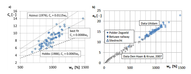
[7]	Den Haan EJ, Kruse GAM (2007) Characterisation and engineering properties of Dutch peats. In Second international workshop on characterisation and engineering of natural soils Singapore, London Taylor & Francis, 3: 2101-2133.
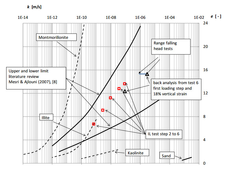
[8]	Mesri G, Ajlouni M (2007) Engineering properties of fibrous peats. J Geotech Geoenviron Eng 133: 850-866.
[9]	Edil TB (2001) Site Characterization in Peat and Organic Soils. Proceedings of International Conference on In Situ Measurement of Soil Properties and Case Histories, Bali, 49-59.
[10]	Helenelund KV (1967) Vane tests and tension tests on fibrous peats. In Proceedings of the Geotechnical Conference on Shear Strength Properties of Natural Soils and Rocks, Oslo Norway, Balkema, Rotterdam, the Netherlands, 19-22.
[11]	Landva AO (2007) Characterization of Escuminac peat and construction on peatland. In Tan TS, Phoon KK, Hight DW, et al. (eds), Characterisation and Engineering Properties of Natural Soils, Taylor& Fransic Group London.
[12]	Boylan N, Long M (2014) Evaluation of peat strength for stability assessments. Geotech Eng 167: 421-430.
[13]	Hobbs NB (1986) Mire Morphology and the properties and behaviour of some British and foreign peats. Q J Eng Geol 19: 7-80. doi: 10.1144/GSL.QJEG.1986.019.01.02
[14]	CROW (Centrum voor Regelgeving en Onderzoek Grond-, Water-, en Wegenbouw) (2015) standaard RAW bepalingen, proef 28 (in Dutch).
[15]	Skempton AW, Petley DJ (1970) Ignition loss and other properties of peats and clays from Avonmouth, King's Lynn and Cranberry Moss. Géotechnique 20: 343-356. doi: 10.1680/geot.1970.20.4.343
[16]	Becker DE, Crooks JHA, Been K, et al. (1987) Work as a criterion for determining in situ and yield stress in clays. Can Geotech J 24: 549-564.
[17]	Azzouz AMRS, Krizek RJ, Corotis RB (1976) Regression analysis of soil compressibility. Soils Found 16: 19-29.
[18]	Casagrande A, Fadum RE (1940) Notes on soil testing for engineering purposes. Harvard Graduate School of Engineering, Soil Mechanics Series No 8, 74.
[19]	ASTM D2435/D2435M-11 (2011) Standard Test Methods for One-Dimensional Consolidation Properties of Soils Using Incremental Loading, ASTM International West Conshohocken, USA.
[20]	Taylor DW (1942) Research on consolidation of clays. Massachusetts Institute of Technology, department of civil engineering, serial no 82.
[21]	Tavenas F, Jean P, Leblond JP, et al. (1983) The permeability of natural soft clays: part Ⅱ: permeability characteristics. Can Geotech J 20: 645-660.
[22]	Yamaguchi H, Ohira Y, Kogure K, et al. (1985) Undrained chear characteristics of normally consolidated peat under triaxial compression. Soils Found 25: 1-18.
[23]	Zwanenburg C, Den Haan EJ, Kruse GAM, et al. (2012) Failure of a trial embankment on peat in Booneschans, the Netherlands. Géotechnique 62: 479-490. doi: 10.1680/geot.9.P.094
[24]	Hendry MT, Sharma JS, Martin CD, et al. (2012) Effect of fibre content and structure on anisotropic elastic stiffness and shear strength of peat. Can Geotech J 49: 403-415. doi: 10.1139/t2012-003
[25]	O'Kelly BC (2017) Measurement, interpretation and recommended use of laboratory strength properties of fibrous peat. Geotech Res 4: 136-171.
[26]	Dyvik R, Lacasse S, Berre T, et al. (1987) Comparison of truly undrained and constant volume direct simple shear tests. Géotechnique 37: 3-10. doi: 10.1680/geot.1987.37.1.3
[27]	Ladd CC, Foot R (1974) New design procedure for stability of soft clays. J Geotech Eng Div 100: 763-786.
[28]	Zwanenburg C (2017) The development of a large diameter sampler. In Proceedings of the 19^th International Conference on Soil Mechanics and Geotechnical Engineering, Seoul.
[29]	Lunne T, Robertson PK, Powell JJM (1997) Cone Penetration Testing in geotechnical practice, Blackie Academic & Professional London.
[30]	Boylan N, Long M, Mathijssen F (2011) In situ strength characterisation of peat and organic soil using full-flow penetrometers. Can Geotech J 48: 1085-1099.
[31]	NEN (2013) NEN EN-ISO 22476-1:2012, IDT Geotechnical investigation and testing-Field testing-Part1: electrical cone and piezocone penetration test. Delft, the Netherlands, NEN.
[32]	Boylan N, Mathijssen F, Long M, et al. (2008) Accuracy of piezocone testing in organic soils. In Proceedings of the 11th Baltic Sea Geotechnical Conference, Gdansk Poland, 1: 367-375.
[33]	Schneider JA, Randolph MF, Mayne PW, et al. (2008) Analysis of factors influencing soil classification using normalized piezocone tip resistance and pore pressure parameters. J Geotech Geoenviron Eng 134: 1569-1586.
[34]	Morris PH, Williams DJ (2000) A revision of Blight's model of field vane testing. Can Geotech J 37: 1089-1098.
[35]	Bjerrum L (1973) Problems of soil mechanics and construction on soft clays and structurally unstable soils (collapsible, expansive and others). Proc. 8th ICSMFE, Moscow, 3: 111-159.

This article has been cited by:

Mahmoud S. Mehany, Faizah D. Alanazi, An

$\eta$ -Hermitian solution to a two-sided matrix equation and a system of matrix equations over the skew-field of quaternions, 2025, 10, 2473-6988, 7684, 10.3934/math.2025352

Reader Comments

Your name:*

Email:*
© 2019 the Author(s), licensee AIMS Press. This is an open access article distributed under the terms of the Creative Commons Attribution License (http://creativecommons.org/licenses/by/4.0)