


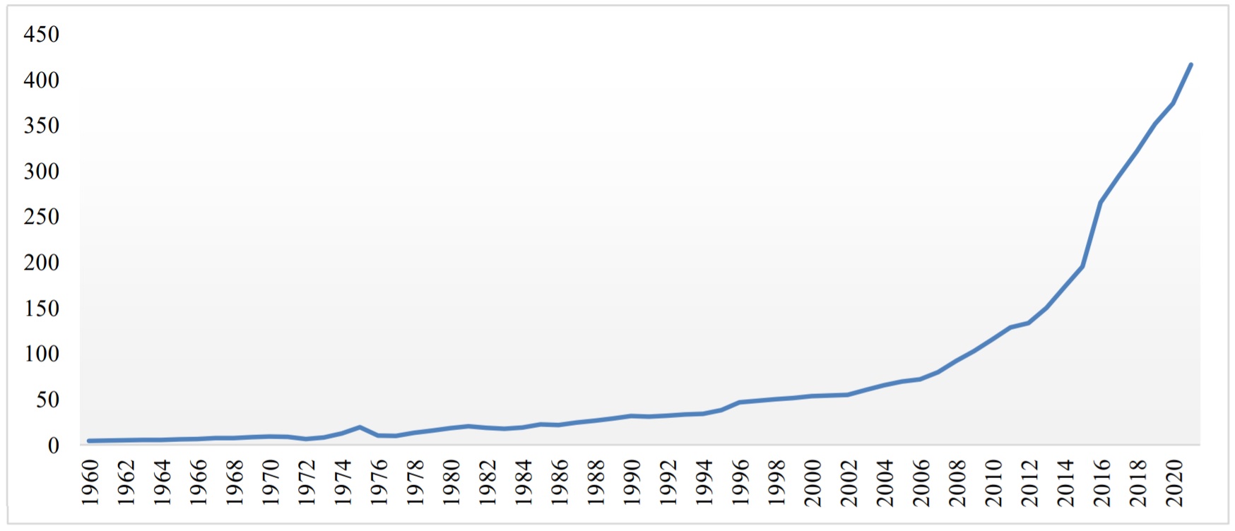
Figure 1.
GDP of Bangladesh.
Note: GDP (constant exchange rate 2015 USD$) in billions (source: The World Bank Group).
Citation: Shailesh Kumar Singh, Nelly Marcy. Comparison of Simple and Complex Hydrological Models for Predicting Catchment Discharge Under Climate Change[J]. AIMS Geosciences, 2017, 3(3): 467-497. doi: 10.3934/geosci.2017.3.467
| [1] | Osarumwense Osabuohien-Irabor, Igor M. Drapkin . FDI Escapism: the effect of home country risks on outbound investment in the global economy. Quantitative Finance and Economics, 2022, 6(1): 113-137. doi: 10.3934/QFE.2022005 |
| [2] | Gerasimos G. Rompotis . The impact of taxation on firm performance and risk: Evidence from Greece. Quantitative Finance and Economics, 2024, 8(1): 29-51. doi: 10.3934/QFE.2024002 |
| [3] | Md Akther Uddin, Mohammad Enamul Hoque, Md Hakim Ali . International economic policy uncertainty and stock market returns of Bangladesh: evidence from linear and nonlinear model. Quantitative Finance and Economics, 2020, 4(2): 236-251. doi: 10.3934/QFE.2020011 |
| [4] | Tolga Tuzcuoğlu . The impact of financial fragility on firm performance: an analysis of BIST companies. Quantitative Finance and Economics, 2020, 4(2): 310-342. doi: 10.3934/QFE.2020015 |
| [5] | Dilvin Taşkın, Görkem Sarıyer . Use of derivatives, financial stability and performance in Turkish banking sector. Quantitative Finance and Economics, 2020, 4(2): 252-273. doi: 10.3934/QFE.2020012 |
| [6] | Ikram Ben Romdhane, Mohamed Amin Chakroun, Sami Mensi . Inflation Targeting, Economic Growth and Financial Stability: Evidence from Emerging Countries. Quantitative Finance and Economics, 2023, 7(4): 697-723. doi: 10.3934/QFE.2023033 |
| [7] | Gigamon Joseph Prah . Innovation and economic performance: The role of financial development. Quantitative Finance and Economics, 2022, 6(4): 696-721. doi: 10.3934/QFE.2022031 |
| [8] | Tinghui Li, Xue Li, Khaldoon Albitar . Threshold effects of financialization on enterprise R & D innovation: a comparison research on heterogeneity. Quantitative Finance and Economics, 2021, 5(3): 496-515. doi: 10.3934/QFE.2021022 |
| [9] | Tânia Menezes Montenegro, Pedro Meira, Sónia Silva . The investors' prospects on mandatory auditor rotation: evidence from Euronext Lisbon. Quantitative Finance and Economics, 2023, 7(3): 440-462. doi: 10.3934/QFE.2023022 |
| [10] | Yue Liu, Yuhang Zheng, Benjamin M Drakeford . Reconstruction and dynamic dependence analysis of global economic policy uncertainty. Quantitative Finance and Economics, 2019, 3(3): 550-561. doi: 10.3934/QFE.2019.3.550 |
Political instability significantly impacts business performance, followed by crime, theft, violence and corruption (Batzilis, 2020; Kirikkaleli, 2020). Emerging-market nations are highly vulnerable to political risk, corruption and violence (Acharya et al., 2015; Diamonte et al., 1996; Marquis & Raynard, 2015). Thus, companies in emerging economies face a tremendous challenge to bear those economic uncertainties, and, recently, COVID-19 fueled the economic uncertainties more (Abdullah et al., 2022). Business organizations play a significant role in the economic development of an emerging economy, and a firm's financial performance and profitability is an essential topic in the finance literature. Researchers, policymakers and regulators always tend to figure out the main driver of and barriers to a firm's financial performance. Many previous studies figured out different firm-specific, industry-specific and macroeconomic determinant factors of a firm's profitability (Abdullah, 2015; Altayligil & Çetrez, 2020; Killins, 2020; Nguyen & Nguyen, 2020). The principal macroeconomic factors figured out by previous studies are the gross domestic product (GDP), inflation, foreign direct investment, taxation system, etc. Few prior studies were set to reveal the impact of political instability on firm performance (Hosny, 2020; Ouà et al., 2020).
Our research is focused on Bangladesh, which is apparently one of the emerging economies with rapid economic growth. As of 2020, Bangladesh's GDP is USD 323.06 billion, which puts it in the 40th position out of 184 countries (source: The World Bank). Moreover, Figure 1 shows that the GDP of Bangladesh has been growing rapidly over the past decade. Additionally, Figure 2 shows that political stability has also been increasing and becoming much more stable over the past decade. For instance, Rahman and Rashid (2018) implied that political stability enhances corporate growth, which eventually increases economic growth through different streams, e.g., price level, tourism sectors, exports and imports of Bangladesh. Overall, this rapid growth of the GDP and stability of the political condition motivated us to examine how firm performance responds to political stability. Empirically, it is unknown how political stability impacts firm performance in Bangladesh.

Existing literature only focuses on how political stability affects different macroeconomic aspects, such as institutional quality (Abreo et al., 2021; Borojo & Yushi, 2020; Bucciol, 2018; Uddin et al., 2020), economic growth (Constantine, 2017; Goldsmith, 1987; Roe & Siegel, 2011; Tiwari, 2013; Uddin & Habibullah, 2013; Uddin et al., 2017b), foreign direct investment (Anyanwu & Yaméogo, 2015; Dupasquier & Osakwe, 2006; Hoque et al., 2018; Kim, 2010; Kurecic & Kokotovic, 2017) and the inflation rate (Tiwari, 2013). However, there is no study in the existing literature that examines the relationship between political stability and firms' financial performance in the context of Bangladesh. Few studies analyzed the effect of political instability on a bank's profitability. Hosny (2017) surveyed 6,083 private firms, and 47% indicated that their growth is hampered by political instability. Yahya et al. (2017) found a positive impact and Athari (2021) found a negative impact of political instability on bank profitability; their findings were not robust, and their sample size was minimal. Moreover, they did not consider panel data methodologies, which provide a more robust estimation. Thus, this study applies a dynamic panel generalized method of moments (GMM) to examine the relationship between political instability and a firm's financial performance. Furthermore, this study covers different firms from different industries, so quantile regression has been applied to test the same hypothesis for the robustness of the results.
Olson's theory suggests that political stability does not affect economic activity up to a certain level. Thus, political stability has a threshold effect on firm's financial performance (Goldsmith, 1987). So, firms operating in emerging economies are habituated to political uncertainty. The question remains: what level of political stability is required for a firm's stable financial performance? No previous study has shown the threshold effect of political stability on a firm's financial performance. The threshold shows the intensity level that is just scarcely visible (Hansen, 1999). Subsequently, this study aimed to find out the threshold of the political stability of Bangladesh.
This study provides several contributions, as follows:
1. It is the first attempt to theoretically and empirically examine the importance of sound political conditions on financial performance in the context of the Bangladesh.
2. This study also examined Olson's theory of a political stability threshold.
3. This study can work as a guide for the emerging economies, as international investors would be able to get an overview of political stability impact performance.
4. For the policymakers, regulators and investors, this study provides evidence of the threshold of political stability on a firm's financial performance.
5. This study also provides some critical policy recommendations for regulators, governments, policymakers and investors.
The rest of the paper is organized as follows. Section 2 provides a brief literature review; Section 3 discusses the data and methodology of this study; Section 4 elaborates the results and findings; Section 5 continues the discussion of the results and presents some policy implications; finally, it ends with Section 6 as the conclusion.
The literature review for this study is divided into two major parts:
1. The role of political stability on the macroeconomic aspect.
2. the role of political stability on firms' aspect.
In the related literature on the macroeconomic aspect, many studies have been conducted to figure out the effect of political stability from an economic perspective, i.e., foreign direct investment (Anyanwu & Yaméogo, 2015; Dupasquier & Osakwe, 2006; Hoque et al., 2018; Kim, 2010; Kurecic & Kokotovic, 2017) and economic growth (Goldsmith, 1987; Roe & Siegel, 2011; Tiwari, 2013; Uddin & Habibullah, 2013; Uddin et al., 2017b). Foreign direct investment is a significant source of capital for local firms. However, Lucas (1990) argued that political instability hinders the foreign investment flow. Focusing on the empirical research on Bangladesh, Chowdhury (2017) showed that, in Bangladesh, the regulatory quality and political stability increase foreign direct investment inflow. Additionally, Das et al. (2021a) showed that institutional quality reduces capital flight in Bangladesh. On the other hand, few studies on African nations found political instability also as a substantial obstacle to foreign capital entry (Anyanwu & Yaméogo, 2015; Dupasquier & Osakwe, 2006). Another study by Kurecic and Kokotovic (2017) applied the Granger causality test and Autoregressive Distributed Lag (ARDL) models to different countries with different political conditions. This study concluded a long-term association between foreign direct investment and political stability in developing economies. Kim (2010) also concluded similar results, i.e., that there is a low flow of foreign direct investment in politically unstable countries, and that there is a high foreign direct investment flow in stable countries. Another group of studies argued that sound political stability increases overall economic growth. Uddin et al. (2017b) applied a dynamic GMM and quantile regression to 120 developing nations' data covering 1996 to 2014 to examine the relationship between economic growth and political stability. This study concluded that Organization of Islamic Cooperation (OIC) countries are much more politically unstable, and that this is creating a massive barrier to economic growth. Another study by Tiwari (2013) examined the impact of political stability on economic growth and the tax system. This study applied quantile regression to 98 countries' unbalanced data and 57 countries' balanced data from 2002 to 2008. This study found that political stability affects the tax system in lower and somewhat higher quantiles, but does not affect the highest and immediate quantiles.
Regarding firm performance, we found a different mix of studies. While the majority of studies have focused on the determinants of a firm's financial performance (Abdullah, 2015; Ahmed et al., 2017; Dietrich & Wanzenried, 2011; Fairfield & Yohn, 2001; Gruszczynski, 2006; Hosny, 2020; Nariswari & Nugraha, 2020; Ouà et al., 2020; Taani & Hamed Banykhaled, 2011), another group of studies focused on the effect of different institutional quality factors on firm performance, i.e., bank performance (Athari, 2021; Yahya et al., 2017) and firm performance (Jens, 2017; Julio and Yook, 2012; (Ahmed et al., 2022; Hillman & Hitt, 1999; Marquis & Raynard, 2015; Zhao, 2012). Uddin et al. (2017a) examined the effect of socio-economic factors on the sector of Bangladesh, and they uncovered that there is no significant association between political stability and bank profitability. However, they posited that there must be some sort of relationship between political stability and bank profitability. A study by Çolak et al. (2017) contended that the ambiguity of the political condition of an economy upsurges the uncertainty of the potential returns from investment. Moreover, firms tend to slow their business expansion process and hold their cash flow due to political instability. Thus, firms incur enormous opportunity costs (Jens, 2017; Julio & Yook, 2012). According to Roe and Siegel (2011), political instability deteriorates financial market development and institutional quality, eventually hindering a firm's financial performance. Moreover, existing literature argues that the degree of successful management of relations with government determines the competitive position operating in weak or unstable circumstances (Hillman & Hitt, 1999; Marquis & Raynard, 2015; Yoffie, 1988).
Besides, according to Marquis and Raynard (2015), the volatility of a firm's financial performance is highly connected to interpersonal networks and personal ties. Thus, a firm always intends to maintain a good relationship with the government by doing different philanthropic activities (Hillman & Hitt, 1999; Marquis & Raynard, 2015; Zhao, 2012). A recent study examined the effects of political risk and global economic policy uncertainty on different banks' profitability based on Ukraine's policy from 2005 to 2015 over a 10-year period. This study found a negative impact of political risks on Ukrainian banks (Athari, 2021). Yahya et al. (2017) adopted ordinary least square regression to examine the effects of political stability on banks' profitability by using the data from 2010 to 2014 in Yemen. This study argued that political stability has a negative effect on Yemeni banks' profitability. Thus, this result contradicts the result of Athari (2021). Moreover, both studies did not consider the dynamic panel and quantile regression models or different industry data. Shaddady (2021) suggested that an organization's primary objective is to reduce the uncertainty and risks related to political instability. Moreover, political stability decreases the degree of economic uncertainty, which eventually assists the business development process. Economic uncertainty increases production and transaction costs, reducing business profitability (Borojo & Yushi, 2020). Governmental stability creates the conditions for businesses to succeed and grow by fostering improved business confidence through stable, predictable and dependable political processes. With a transparent power transition of governments, a favorable environment for businesses to grow is created (Manolova et al., 2008). Petracco and Schweiger (2012) analyzed the effect of the conflict between Russia and Georgia in 2008 on firms' sales. This study found a significant negative impact of political instability on firms' sales and export.
Moreover, Hosny (2020) examined the effects of political instability on firm performance by using firm-level data covering 592 firms in Tunisia; they found a negative association. Another study used a survey of 361 firms in the Ivory Coast to examine the microeconomic impact of political instability on firm performance in the Ivory Coast. This study found a negative relationship with firm performance (Ouà et al., 2020). Another study surveyed 80 firms to determine the barriers to a firm's growth (Ayyagari et al., 2008). Many respondents of this study argued that political instability directly hinders the firm's growth. Another study by Avina (2013) argued that the profitability of many firms decreased due to the political instability in the Arab countries. Another study by Hoque et al. (2018) argued about the endogeneity among stock market development and foreign direct investment with the moderating effect of political instability. This study employed ARDL and a hierarchical regression approach by using the data from 1993 to 2016 in Bangladesh. It found negative long-run and short-run moderating effects on stock market development. Roxas et al. (2012) applied logistics regression to the business performance index data of 751 companies in South Africa. They found an insignificant negative association between business performance and political instability. A recent study by Gaganis (2019) analyzed 40,000 small and medium-sized enterprise (SME) firms' data from 25 European Union countries' data covering the period from 2006 to 2014. This study argued that a corruption-free economy is a primary condition for sound business, and that corruption is reduced by stable political conditions. Overall, the literature only contains a few bank's performance-related studies on political stability with unclear results, and there is no evidence on firms' financial performance, particularly in Bangladesh. Consequently, the above arguments show that the stable political condition of a country is favorable for the daily operations of firms. Thus, we present the following hypothesis:
H1: There is a positive association between political stability and a firm's financial performance.
However, the effect of political stability on a firm's financial performance might be nonlinear. According to Max Weber's theory, the government's authorized use of physical force is necessary for political stability. Suppose that the government is unable to provide fundamental services to its citizens, such as security and the capacity to obtain food and shelter. In that case, it loses its authority to enforce laws, resulting in political instability (Wolin, 1981). Political stability reduces corruption and other barriers to a firm's financial performance (Diamonte et al., 1996; Kurecic and Kokotovic, 2017). According to Olson's theory, political instability and stability are dichotomous. Political stability starts boosting the economy after a threshold. Subsequently, lower political stability does not affect economic activity (Goldsmith, 1987). Thus, based on Olson's theory, the following hypothesis was developed:
H2: There is a threshold effect of political stability on a firm's financial performance.
Overall, the above literature highlighted that political stability has an impact at the macroeconomic and firm levels. However, it is still inconclusive on how domestic-level political stability affects the firm performance, and on the nonlinear or threshold effect of political stability on firm performance. Therefore, in light of these knowledge gaps, this study contributes to the literature by adding new empirical evidence through the use of linear and nonlinear analysis.
This study aimed to inspect the effects of political stability on a firm's financial performance. Emerging market firms are more vulnerable to political risk factors (Diamonte et al., 1996; Marquis & Raynard, 2015). However, over the past decade, the political stability of Bangladesh has been increasing. Therefore, we selected Bangladesh as a sample country. We collected the firm-related data from the Refinitiv Datastream database, where 360 Bangladeshi firms have data available. However, most of them have been added recently, and there are many missing values. Thus, based on the data available at Refinitiv Datastream, and with the aim of covering as many companies and years as possible, we selected 139 firms in Bangladesh and a sample period covering the period from 2011 to 2020. The selected variables and their data sources are described in Table 1. The dependent variable, i.e., the return on assets (ROA), was taken as the proxy for the firm financial performance. Political stability is the independent variable measured through the proxy "Political Stability and Absence of Violence/Terrorism" of worldwide governance indicators from The World Bank, and it can be described as follows: "Political Stability and Absence of Violence/Terrorism measures perceptions of the likelihood of political instability and/or politically motivated violence, including terrorism" (WGI, 2020). Moreover, this study applied the methodology of Altman and Hotchkiss (2010) to calculate the Altman Z-Score (Z). The Altman Z-score is the estimation of the likelihood of a publicly traded firm's solvency.
| Variables | Definition | Calculation | Reference | Data Source | |
| Dependent Variable: | |||||
| ROA | Return on assets (ROA) is a financial ratio that shows how profitable a business is in relation to its total assets. | (Net Income / Total Assets)*100 | Athari, 2021; Gaganis et al., 2019 | Refinitiv Datastream | |
| Independent Variable: | |||||
| PS | Political Stability and Absence of Violence/Terrorism is the percentile rank term of the likelihood of political instability and/or politically motivated violence, including terrorism, ranging from 0 (lowest rank) to 100 (highest rank) | * | Tiwari, 2013; Uddin et al., 2017b | World Governance Indicators, The World Bank | |
| Firm-Specific Variables: | |||||
| SIZE | Firm Size | Natural Logarithm (Total Assets) | Dietrich & Wanzenried, 2011 | Refinitiv Datastream | |
| LEV | Leverage | Total Liabilities/ Total Equities | Athari, 2021; Gaganis et al., 2019 | Refinitiv Datastream | |
| EPS | Earnings per share refer to the monetary value of a company's earnings per outstanding share of common stock. | (Net Income-Preferred Dividend) / Shares Outstanding | Dietrich and Wanzenried, 2011 | Refinitiv Datastream | |
| Z | The Altman Z-score is the result of a credit-strength test that determines the likelihood of a publicly traded company going bankrupt. | See Altman & Hotchkiss (2010) | Abdullah, 2021 | Refinitiv Datastream | |
| NPM | Profit margin is a measure of profitability. | (Net Income/ Revenue)*100 | Nariswari and Nugraha, 2020 | Refinitiv Datastream | |
| MVBV | The market-to-book value ratio compares the market value of a company with its book value. | Market Value/Book Value | Abdullah, 2015; Gan et al., 2020 | Refinitiv Datastream | |
| Note: *: see http://info.worldbank.org/governance/wgi/Home/Documents#wgiAggMethodology for the calculation methodology for Political Stability and Absence of Violence/Terrorism. | |||||
 DownLoad:
CSV
DownLoad:
CSV
To test the first hypothesis, we employed static and dynamic panel regressions. Moreover, we have employed dynamic panel quantile regressions to examine the robustness of the static and dynamic models, where quantile regression considers regression over conditional distribution. Finally, to test our second hypothesis, we employed threshold regression. Further details of each method are elaborated on in the following subsections.
According to different scholars' opinions, the dynamic panel data GMM is more efficient because it uses more determinant factors and features (Arellano and Bond, 1991; Hayakawa et al., 2007; Uddin et al., 2020). The lagged effect should be considered as a determination of the firms' indicators, which could affect their next year's performance (Uddin et al., 2020). This study also argued that the correlation between predictors and lagged independent variables, unobserved endogeneity and heterogeneity indicates that fixed- or random-effects models may not be suitable for the estimation of balanced panel data. For this instance, we applied the dynamic system GMM suggested by Arellano and Bond (1991) and Hansen (1982). The equation for the GMM is as follows:
| Yi,t=αYi,t−1+β1Xi,t+β2Zi,t+μi+ϵi,t | (1) |
Here, Yi,t denotes the dependent variables, Yi,t−1 denotes the dependent variables in the year t−1, Xi is a vector of independent variables, Zi is a vector of firm specific explanatory variables, μi is the firm-specific time-invariant effect which allows for heterogeneity across firms and ϵi,t is the error term.
The sample of this study consisted of industries with different levels of firm sizes and different levels of operational exposure. For example, the bank's asset size is larger, and their area of operations covers the full country. Subsequently, ordinary least squares were applied to consider only normally distributed error, which is an assumption that is not correct for this study sample, as political stability and other variables follow a skewed distribution. Moreover, the variables were from different industries' firms, and they consisted of outliers and heavy-tailed distributions because their sizes are different. In this case, quantile regression output more robust results than the ordinary least square regression model.
Additionally, ordinary least square regression models only consider the mean, but quantile regressions can explain the whole conditional distribution of the outcome variable (Das et al., 2021b; Tiwari, 2013). By following the quantile regression model of Koenker (2004) and Baker (2016), we applied dynamic quantile regression to examine whether different stages of firm performance are affected by political stability and other firm-specific variables. Thus, the dynamic quantile regression can be written as:
| yit=β0yi,t−1+x'itβ1+ϵitQuantθ(yitxit)=x'itβ0(U∗it) | (2) |
Here, t denotes time, i denotes a firm, yit denotes firm performance, yi,t−1 denotes the lagged firm performance, x'it denotes the vector of political stability and firm-specific variables, β denotes the vector of factors to be calculated and ε denotes the error term. Quantθ denotes the conditional quantile, whereas the general disturbance term is denoted by U.
Finally, this study aimed to conduct a threshold analysis to determine the threshold level of political stability for the standard level of firm performance. Dynamic threshold regression analysis was estimated for one threshold value of political stability for the threshold analysis. Equation 3 describes the model of threshold regression, which has been derived from Seo and Shin (2016).
| yit=αi+δx'it+k(qit−γ)1{qit>γ}+ϵit | (3) |
Here, yit denotes the dependent variable firm performance, and the threshold variable is defined as qit; γ denotes the threshold value, x'it indicates the explanatory and lagged dependent variables and ϵi,t indicates the error term.
The results of descriptive statistics and correlation analysis are presented in Table 2. The results of the descriptive statistics denote that LEV, NPM and EPS are highly volatile, as the standard deviations were 9.68, 18.55 and 11.12, respectively. As this data consist of different sizes of industries and differently sized firms, this volatility is expected. The mean size was 23.66 for the sampled companies. Nevertheless, the mean value of EPS denotes that few companies performed better in terms of stock performance. Almost all variables were positively skewed, except the ROA and NPM.
| Variables | ROA | SIZE | LEV | NPM | EPS | MVBV | Z | PS |
| N | 1,390.00 | 1,390.00 | 1,390.00 | 1,390.00 | 1,390.00 | 1,390.00 | 1,390.00 | 1,390.00 |
| Mean | 6.67 | 23.66 | 5.38 | 16.89 | 6.91 | 1.45 | 0.94 | 11.94 |
| SD | 8.22 | 1.83 | 9.68 | 18.55 | 11.12 | 2.08 | 1.19 | 3.12 |
| Min | −3.18 | 18.23 | −26.25 | −5.34 | 0.01 | 0.04 | −2.33 | 7.58 |
| Max | 31.81 | 27.98 | 139.85 | 74.17 | 46.22 | 8.51 | 4.02 | 16.67 |
| SKW | 1.45 | −0.05 | 7.2 | 1.5 | 2.63 | 2.19 | 0.11 | 0.28 |
| KRT | 4.53 | 2.3 | 83.1 | 5.1 | 9.15 | 7.26 | 4.64 | 1.57 |
| Variables | ROA | SIZE | LEV | NPM | EPS | MVBV | Z | PS |
| ROA | 1.00 | |||||||
| SIZE | 0.19*** | 1.00 | ||||||
| LEV | −0.29*** | −0.18*** | 1.00 | |||||
| EPS | 0.47*** | 0.06** | −0.08*** | 1.00 | ||||
| Z | 0.37*** | 0.15*** | −0.28*** | 0.24*** | 1.00 | |||
| NPM | 0.54*** | 0.16*** | −0.04 | 0.59*** | 0.26*** | 1.00 | ||
| MVBV | 0.35*** | 0.01 | −0.15*** | 0.25*** | 0.23*** | 0.35*** | 1.00 | |
| PS | 0.08*** | 0.04* | −0.01 | 0.04* | 0.09*** | −0.01 | −0.07*** | 1.00 |
| Note: N= Number of Observations, SD= Standard Deviation Min= Minimum, Max= Maximum, SKW= Skewness, KRT= Kurtosis, Significance levels: *** p < 0.01, ** p < 0.05, * p < 0.1. | ||||||||
DownLoad:
CSV
Furthermore, Pearson correlation analysis was conducted to examine the correlations among the variables. Table 2 indicates a significant positive correlation between the dependent variable financial performance (ROA) and the primary independent variable political stability (PS). Other variables had a statistically significant positive correlation with ROA, except LEV. Previous studies also found a similar association between financial performance and firm-specific variables (Abdullah, 2015; Ahmed et al., 2017; Dietrich & Wanzenried, 2011; Fairfield & Yohn, 2001; Gruszczynski, 2006; Nariswari & Nugraha, 2020; Taani & Hamed Banykhaled, 2011).
At first, static models, i.e., pooled ordinary least squares (OLS), fixed-effects and random-effects regressions, were analyzed to check the validity of the dynamic model; finally, seven dynamic GMMs were developed as a result of the inclusion and exclusion of firm-specific variables in the model; the results are presented in Table 3. The results of pooled OLS, fixed-effects and random-effects regressions show that there is a significant positive impact of political stability on firm performance. Specification tests were conducted to compare the static model, and the results are presented in Table A.1 (Appendix A). The Breusch-Pagan Lagrangian multiplier test null hypothesis was that the random-effects variance was zero, and the p-value rejected the null hypothesis and suggested random effects. Moreover, the results of the Hausman test of the fixed-effects vs. random-effects and fixed-effects vs. pooled OLS p-value rejected the null hypothesis and suggested that the fixed-effects model is better; and, the ui = 0 F-test p-value showed the fitness of the fixed-effects model. However, the Wooldridge serial correlation test p-value results rejected the null hypothesis of no serial correlation. This test result indicates that serial correlation existed in our static models; thus, finally, we shall move to dynamic panel models.
| Variables | POLS | FE | RE | GMM 1 | GMM 2 | GMM 3 | GMM 4 | GMM 5 | GMM 6 | GMM 7 |
| L.ROA | 0.434*** | 0.435*** | 0.493*** | 0.385*** | 0.479*** | 0.447*** | 0.470*** | |||
| (0.048) | (0.048) | (0.045) | (0.051) | (0.048) | (0.051) | (0.053) | ||||
| SIZE | 0.304*** | 0.267*** | 0.296*** | 0.215*** | 0.264*** | 0.218*** | 0.235*** | 0.246*** | 0.133* | |
| (0.094) | (0.081) | (0.089) | (0.071) | (0.073) | (0.070) | (0.070) | (0.075) | (0.070) | ||
| LEV | −0.167*** | −0.049*** | −0.133*** | −0.107*** | −0.107*** | −0.109*** | −0.123*** | −0.109*** | −0.100*** | |
| (0.018) | (0.018) | (0.019) | (0.020) | (0.020) | (0.021) | (0.020) | (0.020) | (0.022) | ||
| EPS | 0.140*** | −0.091*** | 0.116*** | 0.042** | 0.045** | 0.040** | 0.035 | 0.089*** | −0.032 | |
| (0.019) | (0.027) | (0.022) | (0.020) | (0.020) | (0.020) | (0.022) | (0.021) | (0.022) | ||
| Z | 0.894*** | 0.630*** | 0.754*** | 0.785*** | 0.819*** | 0.987*** | 0.833*** | 0.877*** | 0.723*** | |
| (0.153) | (0.150) | (0.156) | (0.164) | (0.162) | (0.157) | (0.166) | (0.165) | (0.166) | ||
| NPM | 0.147*** | 0.043*** | 0.095*** | 0.063*** | 0.063*** | 0.055*** | 0.080*** | 0.073*** | 0.142*** | |
| (0.012) | (0.012) | (0.012) | (0.013) | (0.012) | (0.013) | (0.012) | (0.012) | (0.021) | ||
| MVBV | 0.534*** | −0.535*** | 0.163* | 0.335*** | 0.318*** | 0.280*** | 0.385*** | 0.352*** | 0.451*** | |
| (0.087) | (0.092) | (0.091) | (0.075) | (0.072) | (0.092) | (0.078) | (0.075) | (0.086) | ||
| PS | 0.163*** | 0.158*** | 0.153*** | 0.049* | 0.046* | 0.051* | 0.056** | 0.060** | 0.049* | 0.047* |
| (0.054) | (0.042) | (0.047) | (0.026) | (0.026) | (0.026) | (0.026) | (0.029) | (0.028) | (0.027) | |
| Constant | −6.647*** | −1.175 | −4.801** | −4.010** | 1.058** | −6.155*** | −3.960** | −4.213** | −4.315** | −2.560 |
| (2.291) | (1.966) | (2.168) | (1.741) | (0.473) | (1.702) | (1.703) | (1.681) | (1.862) | (1.728) | |
| Observations | 1,390 | 1,390 | 1,390 | 1,251 | 1,251 | 1,251 | 1,251 | 1,251 | 1,251 | 1,251 |
| Year and firm fixed effects | Yes | Yes | Yes | |||||||
| R-squared | 0.441 | 0.091 | ||||||||
| Number of Firms | 139 | 139 | 139 | 139 | 139 | 139 | 139 | 139 | 139 | 139 |
| Serial correlation | 0.000 | |||||||||
| AR(1) | 0.000 | 0.000 | 0.000 | 0.000 | 0.000 | 0.000 | 0.000 | |||
| AR(2) | 0.624 | 0.652 | 0.549 | 0.682 | 0.555 | 0.829 | 0.388 | |||
| Hansen | 0.106 | 0.134 | 0.0748 | 0.173 | 0.153 | 0.103 | 0.0792 | |||
| Number of Instruments | 37 | 36 | 36 | 36 | 36 | 36 | 36 | |||
| Note: STATA Command: xtabond2 two-step system GMM, Dependent variables= Firm Financial Performance (ROA), POLS= Pooled Ordinary Least Square, FE= Fixed Effects, RE= Random Effects, Serial correlation= Wooldridge Serial Correlation Test P-Value, Hansen = Hansen Test P-Value. Significance levels: *** p < 0.01, ** p < 0.05, * p < 0.1; Standard errors are in parentheses and second-order autocorrelations of errors are rejected. | ||||||||||
DownLoad:
CSV
The results of the GMM estimator revealed that, for Model 1, political stability had a significant positive impact on a firm's financial performance. Other firm-specific variables had a significant positive impact on an individual firm's financial performance, except LEV. The diagnostic test p-values (AR(1), AR(2), Hansen test) indicate that GMMs are reasonably well specified. The over-identification restrictions were not rejected by the Hansen test or the absence of a second-order serial correlation. There was no instrument proliferation of estimations because the number of instruments was less than the number of cross-sectional dimensions. Moreover, the lag effect of the ROA was significant throughout all models. Considering all of the statistical test results of all models, this study indicated that all models were statistically significant. Our results show that LEV is negatively associated with firm performance, which is the expected outcome, as high leverage works as a double-edged sword. Relating to our results, prior studies suggest that investors always tend to get a higher EPS from their invested firms, that firm size is positively related with firm performance and that the size and EPS positively affect their financial performance (Dietrich & Wanzenried, 2011; Taani & Hamed Banykhaled, 2011).
Furthermore, we used the Worldwide Governance Indicators' political stability and absence of violence data as the proxy for political stability (PS). We found a statistically positive impact of political stability on individual firms' financial performance. This result indicates that, if political stability increases by one point, this will increase the firm's financial performance by 0.046 units of the sampled firms. According to Goldsmith (1987), the theory of Olson argues that political instability and stability are dichotomous, and political stability starts boosting the economy after reaching a threshold. The results of this study are consistent with those of previous studies (Jens, 2017; Julio & Yook, 2012; Kim, 2010; Uddin et al., 2017b; Zhao, 2012). Therefore, this supports the hypothesis of this study, i.e., that political stability positively affects a firm's financial performance.
The dataset of this study comprised different industries' firms, and the values of their variables differ from each other; it has been validated by using descriptive statistics standard deviation values (Tiwari, 2013; Uddin et al., 2017b). To check the robustness, quantile regression was applied to Model 1 of the GMM. The results of quantile regressions are presented in Table 4. This study considered 10% to 90% in the 10% interval interquartile range for quantile regression. The outputs for all variable quantiles are presented in Table 4 and Figure 3. The results indicate that there is a statistically significant positive effect of political stability on the small-sized to large-sized firm's financial performance. Across all quantiles (10% to 90%), political stability had a significant impact on individual Bangladeshi firms' financial performance, similar to GMM 1.
| Q (10) | Q (20) | Q (30) | Q (40) | Q (50) | Q (60) | Q (70) | Q (80) | Q (90) | |
| L.ROA | 0.067*** | 0.396*** | 0.608*** | 0.694*** | 0.805*** | 0.788*** | 0.774*** | 0.754*** | 0.692*** |
| (0.004) | (0.002) | (0.001) | (0.015) | (0.001) | (0.007) | (0.002) | (0.003) | (0.007) | |
| SIZE | 0.443*** | 0.503*** | 0.368*** | 0.103*** | 0.216*** | 0.159*** | 0.244*** | 0.267*** | 0.069* |
| (0.016) | (0.007) | (0.003) | (0.009) | (0.002) | (0.015) | (0.005) | (0.004) | (0.039) | |
| LEV | −0.059*** | −0.056*** | −0.054*** | −0.057*** | −0.060*** | −0.062*** | −0.059*** | −0.058*** | −0.087*** |
| (0.004) | (0.003) | (0.000) | (0.002) | (0.000) | (0.004) | (0.001) | (0.001) | (0.007) | |
| EPS | 0.036*** | 0.014*** | 0.048*** | −0.010 | 0.011*** | −0.001 | 0.006*** | −0.016*** | −0.049*** |
| (0.004) | (0.003) | (0.000) | (0.011) | (0.001) | (0.004) | (0.002) | (0.000) | (0.007) | |
| Z | 0.463*** | 0.471*** | 0.253*** | 0.360*** | 0.497*** | 0.455*** | 0.720*** | 0.794*** | 1.371*** |
| (0.020) | (0.026) | (0.005) | (0.007) | (0.008) | (0.020) | (0.009) | (0.008) | (0.041) | |
| NPM | 0.041*** | 0.039*** | 0.028*** | 0.014*** | 0.025*** | 0.049*** | 0.054*** | 0.050*** | 0.064*** |
| (0.002) | (0.003) | (0.000) | (0.005) | (0.000) | (0.001) | (0.001) | (0.001) | (0.006) | |
| MVBV | −0.010 | 0.041** | 0.073*** | 0.029*** | 0.278*** | 0.176*** | 0.430*** | 0.779*** | 0.800*** |
| (0.014) | (0.017) | (0.001) | (0.005) | (0.004) | (0.018) | (0.011) | (0.006) | (0.024) | |
| PS | 0.040** | 0.031*** | 0.015*** | 0.071*** | 0.021*** | 0.025*** | 0.029*** | 0.088*** | 0.300*** |
| (0.018) | (0.005) | (0.002) | (0.021) | (0.002) | (0.009) | (0.004) | (0.002) | (0.029) | |
| Observations | 1,251 | 1,251 | 1,251 | 1,251 | 1,251 | 1,251 | 1,251 | 1,251 | 1,251 |
| Number of groups | 139 | 139 | 139 | 139 | 139 | 139 | 139 | 139 | 139 |
| Note: STATA Command: qregpd quantile (0.10, 0.20, 0.30, 0.40, 0.50, 0.60, 0.70, 0.80, 0.90); Dependent variable= Firm Financial Performance (ROA), Significance levels: *** p < 0.01, ** p < 0.05, * p < 0.1; Standard errors in parentheses. | |||||||||
DownLoad:
CSV

SIZE, NPM and Z were found to have a statistically positive relationship on a firm's financial performance. MVBV had a significant positive impact across all quantiles, except its negative impact for the 10% quantile. Nevertheless, LEV had a significant negative relationship with financial performance across all quantiles. The positive association between firm financial performance and political stability across the lower-to-upper quantiles in the quantile regression estimator validates that the GMMs and results are robust. Previous studies also found similar associations with political stability (Hoque et al., 2018; Petracco & Schweiger, 2012; Uddin et al., 2017b).
The last objective of this study was to find out the threshold for political stability impact on financial performance. The dynamic panel threshold regression estimator results are presented in Table 5. The bootstrapped linearity test p-value is significant at the 10% level, indicating a significant threshold effect. The p-value (0.000) of the threshold coefficient (γ) is statistically significant and rejects the null hypothesis. Thus, the results indicate a threshold effect of political stability on a firm's financial performance, and the threshold for political stability was found to be 13.680. Before the threshold level of PS (13.680), PS had negative impact on the ROA, and beyond the threshold, it became positive. Interestingly, the results show significant implication of LEV, where, before the threshold level, LEV shows a negative impact, whereas, beyond the threshold level, there is a positive effect. This result indicates that, under sound political conditions, a firm can utilize their debt properly. Among other variables, beyond the threshold level, the effects of SIZE and Z on the ROA increased significantly.
| Variables | PS<13.680 (Before Threshold) |
PS>13.680 (Beyond Threshold) |
| L.ROA | 0.061*** | 0.059*** |
| (0.002) | (0.003) | |
| SIZE | 0.065*** | 0.289*** |
| (0.011) | (0.005) | |
| LEV | −0.056*** | 0.055*** |
| (0.001) | (0.002) | |
| EPS | −0.111*** | −0.014*** |
| (0.001) | (0.001) | |
| Z | 0.375*** | 0.500*** |
| (0.009) | (0.015) | |
| NPM | −0.010*** | −0.006*** |
| (0.001) | (0.001) | |
| MVBV | −0.248*** | −0.458*** |
| (0.005) | (0.004) | |
| PS | −1.632*** | 0.190*** |
| (0.035) | (0.008) | |
| Constant | 23.616*** | |
| (0.539) | ||
| γ | 13.680*** | |
| (0.062) | ||
| Number of Group | 139 | |
| T | 10 | |
| Linearity Test P-Value | 0 | |
| Note: Stata: xthenreg grid_num (100) trim_rate (0.1) boost (500), Coef. = Coefficients, SE = Standard Errors, CI = Confidence Interval, Significance levels: *** p < 0.01, ** p < 0.05, * p < 0.1. | ||
DownLoad:
CSV
This result indicates that, if political stability becomes lower than 13.680, this will decrease a firm's financial performance by 1.62 points, whereas, if PS becomes higher than 13.680, the firm's financial performance will be increased by 0.190 points. So, 13.680 is the threshold level for political stability to increase profitability. Therefore, this study shows a threshold effect of political stability on a firm's financial performance, which also supports Olson's theory (Goldsmith, 1987).
This result indicates that, if political stability becomes lower than 13.680, this will decrease a firm's financial performance by 1.62 points, whereas, if PS becomes higher than 13.680, the firm's financial performance will be increased by 0.190 points. So, 13.680 is the threshold level for political stability to increase profitability. Therefore, this study shows a threshold effect of political stability on a firm's financial performance, which also supports Olson's theory (Goldsmith, 1987).
By applying the dynamic panel GMM, we found that firm-specific variables positively impact a firm's profitability. The literature supports this finding, as previous studies found similar results (Abdullah, 2015; Ahmed et al., 2017; Dietrich & Wanzenried, 2011; Fairfield & Yohn, 2001; Gruszczynski, 2006; Nariswari & Nugraha, 2020; Taani & Hamed Banykhaled, 2011). We developed seven models by including and excluding firm-specific variables and found that political stability has a positive, statistically significant impact on firms' profitability. Our result is consistent with those of earlier studies (e.g., Hosny, 2020; Ouà et al., 2020). This result also supports Olson's theory of political stability (Goldsmith, 1987). Subsequently, the results indicate that, if political stability increases by one point, this will increase the financial performance by 0.046 units. Previous studies found similar associations between political stability and different variables (Jens, 2017; Julio & Yook, 2012; Kim, 2010; Uddin et al., 2017b; Zhao, 2012).
We also applied the quantile regression approach, as the sample consisted of differently sized firms from different industries (Tiwari, 2013). The study yielded robust results across the lower-to-upper quantiles (10% to 90%) and indicates a statistically significant positive impact of political stability on a firm's financial performance. A previous study on another emerging nation also found a similar asymmetric effect, which varied across firm sizes (Rashid et al., 2021). Olson's theory revealed that political stability does not affect economic activity up to a certain level. So, political stability has a threshold effect on a firm's financial performance (Goldsmith, 1987). To find out the threshold for political stability, we applied a dynamic panel threshold model. It revealed that there is a threshold effect of political stability on a firm's financial performance. The threshold for political stability was found to be 13.680, and this result signifies that, if political stability becomes lower than 13.680, this will drastically deteriorate the firm's financial performance. So, 13.680 is the threshold level of political stability that helps to boost economic activity. Therefore, we recommend that the government, regulators and other stakeholders improve political stability to increase business performance. Investors should also implement rigorous investment strategies to increase their performance.
We applied dynamic GMMs and dynamic quantile regression to examine the impact of political stability on a firm's financial performance by using 139 companies from the Dhaka Stock Exchange ranging from 2011 to 2020. We found a statistically significant positive impact of political stability on a firm's financial performance by using a dynamic GMM; the results were robust as a result of using dynamic panel quantile regression. Olson's theory argues that there is a threshold effect for political stability. Subsequently, we applied a panel threshold regression model and found that Bangladesh's political stability threshold is 13.680. The results of our study also revealed that additional points of political stability beyond the threshold has a positive and significant impact on the firm performance. So, this indicates that a higher level of political stability is required to boost the firm performance in Bangladesh. This study has its limitations, such as not considering more countries in the sample. Therefore, we recommend that future studies consider more sample countries and cover an extensive timeline. Future studies can examine the impact of political stability on fintech progress and financial inclusion.
All authors declare no conflicts of interest regarding this paper.
| [1] | Martínez-Santiago S, López-Santos A, González-Cervantes G, et al. (2017) Evaluating the impacts of climate change on soil erosion rates in central mexico. AIMS Geosci 3: 327-351. |
| [2] | Orth R, Staudinger M, Seneviratne SI, et al. (2015) Does model performance improve with complexity? A case study with three hydrological models. J Hydrol 523: 147-159. |
| [3] | Singh SK (2016) Long-term streamflow forecasting based on ensemble streamflow prediction technique: A case study in new zealand. Water Resour Manag 30: 2295-2309. |
| [4] | Michaud J, Sorooshian S (1994) Comparison of simple versus complex distributed runoff models on a midsized semiarid watershed. Water Resour Res 30: 593-605. |
| [5] |
Ludwig R, May I, Turcotte R, et al. (2009) The role of hydrological model complexity and uncertainty in climate change impact assessment. Adv Geosci 21: 63-71. doi: 10.5194/adgeo-21-63-2009

|
| [6] | Graham LP, Andréasson J, Carlsson B (2007) Assessing climate change impacts on hydrology from an ensemble of regional climate models, model scales and linking methods–a case study on the lule river basin. Clim Change 81: 293-307. |
| [7] | Bergström S, Carlsson B, Gardelin M, et al. (2001) Climate change impacts on runoff in sweden-assessments by global climate models, dynamical downscaling and hydrological modelling. Clim res 16: 101-112. |
| [8] | Xu C.-y. (1999) Climate change and hydrologic models: A review of existing gaps and recent research developments. Water Resour Manag 13: 369-382. |
| [9] | Menzel L, Bürger G (2002) Climate change scenarios and runoff response in the mulde catchment (southern elbe, germany). J Hydrol 267: 53-64. |
| [10] | Akhtar M, Ahmad N, Booij MJ (2008) The impact of climate change on the water resources of hindukush–karakorum–himalaya region under different glacier coverage scenarios. J Hydrol 355: 148-163. |
| [11] | Teutschbein C, Seibert J (2012) Bias correction of regional climate model simulations for hydrological climate-change impact studies: Review and evaluation of different methods. J Hydrol 456: 12-29. |
| [12] | Hattermann F, Krysanova V, Gosling SN, et al. (2017)Cross‐scale intercomparison of climate change impacts simulated by regional and global hydrological models in eleven large river basins. Clim Change 141: 561-576. |
| [13] |
Najafi M, Moradkhani H, Jung I (2011) Assessing the uncertainties of hydrologic model selection in climate change impact studies. Hydrol process 25: 2814-2826. doi: 10.1002/hyp.8043
|
| [14] | Bastola S, Murphy C, Sweeney J (2011) The role of hydrological modelling uncertainties in climate change impact assessments of irish river catchments. Adv Water Resour 34: 562-576. |
| [15] | Steinschneider S, Wi S, Brown C (2015) The integrated effects of climate and hydrologic uncertainty on future flood risk assessments. Hydrol Process 29: 2823-2839. |
| [16] |
Seiller G, Anctil F (2014) Climate change impacts on the hydrologic regime of a canadian river: Comparing uncertainties arising from climate natural variability and lumped hydrological model structures. Hydrol Earth Syst Sci 18: 2033. doi: 10.5194/hess-18-2033-2014
|
| [17] |
Oyerinde GT, Wisser D, Hountondji FC, et al. (2016) Quantifying uncertainties in modeling climate change impacts on hydropower production. Clim 4: 34. doi: 10.3390/cli4030034
|
| [18] |
Mango LM, Melesse AM, McClain ME, et al. (2011) Land use and climate change impacts on the hydrology of the upper mara river basin, kenya: Results of a modeling study to support better resource management. Hydrol Earth Syst Sci 15: 2245. doi: 10.5194/hess-15-2245-2011
|
| [19] | Zhang X, Srinivasan R, Hao F (2007) Predicting hydrologic response to climate change in the luohe river basin using the swat model. Transactions of the ASABE 50: 901-910. |
| [20] |
Jasper K, Calanca P, Gyalistras D, et al. (2004) Differential impacts of climate change on the hydrology of two alpine river basins. Clim Res 26: 113-129. doi: 10.3354/cr026113
|
| [21] |
Middelkoop H, Daamen K, Gellens D, et al. (2001) Impact of climate change on hydrological regimes and water resources management in the rhine basin. Clim change 49: 105-128. doi: 10.1023/A:1010784727448
|
| [22] |
Velázquez J, Schmid J, Ricard S, et al. (2013) An ensemble approach to assess hydrological models' contribution to uncertainties in the analysis of climate change impact on water resources. Hydrol Earth Syst Sci 17: 565. doi: 10.5194/hess-17-565-2013
|
| [23] | Poyck S, Hendrikx J, McMillan H, et al. (2011) Combined snow and streamflow modelling to estimate impacts of climate change on water resources in the clutha river, new zealand. J Hydrol (New Zealand) 293-311. |
| [24] | Lawrence J, Reisinger A, Mullan B, et al. (2013) Exploring climate change uncertainties to support adaptive management of changing flood-risk. Environ Sci Policy 33: 133-142. |
| [25] | Gawith D, Kingston DG, McMillan H (2012) The effects of climate change on runoff in the lindis and matukituki catchments, otago, new zealand. J Hydrol (New Zealand) 121-135. |
| [26] |
Jiang T, Chen YD, Xu C.-y., et al. (2007) Comparison of hydrological impacts of climate change simulated by six hydrological models in the dongjiang basin, south china. J hydrol 336: 316-333. doi: 10.1016/j.jhydrol.2007.01.010
|
| [27] | NIWA (2013) Overview of new zealand climate. Available from: Https://www.Niwa.Co.Nz/climate/summaries/annual/annual-climate-summary-2013. |
| [28] |
Tait A, Henderson R, Turner R, et al. (2006) Thin plate smoothing spline interpolation of daily rainfall for new zealand using a climatological rainfall surface. Int J Clim 26: 2097-2115. doi: 10.1002/joc.1350
|
| [29] | Snelder TH, Biggs BJF (2002) Multiscale river environment classification for water resources managements1. JAWRA Journal of the American Water Resour Assoc 38: 1225-1239. |
| [30] | Newsome PFJ, Wilde RH, Willoughby EJ (2000) Land resource information system spatial data layers. Landcare Research Technical Report No.84p. |
| [31] | Mullan B, Wratt D, Dean S, et al. (2008) Climate change effects and impacts assessment. A guidance manual for local government. 2nd edition, ministry for the environment, wellington. 149p, Available from: http://www.Mfe.Govt.Nz/sites/default/files/climate-change-effect-impacts-assessment-may08.Pdf. |
| [32] | IPCC (2007) Climate change 2007: Synthesis report. Contribution of working groups i, ii and iii to the fourth assessment report of the intergovernmental panel on climate chnage.(core writing team, pachauri, p.K. And reisinger, a. (eds.)) ipcc, geneva,switzerland, 104pp. |
| [33] | Singh SK, Bárdossy A (2015) Hydrological model calibration by sequential replacement of weak parameter sets using depth function. Hydrol 2: 69-92. |
| [34] | Singh SK (2010) Parameterization of hydrological model in ungauged catchments: A regionalization technique. LAP Lambert Academic Publishing AG & Co KG: Germany, ISBN-13: 978-3838375588. |
| [35] | Andrews F, Croke B, Jakeman A (2011) An open software environment for hydrological model assessment and development. Environmental Modelling & Software 26: 1171-1185. |
| [36] | Jakeman A, Littlewood I, Whitehead P (1990) Computation of the instantaneous unit hydrograph and identifiable component flows with application to two small upland catchments. J hydrol 117: 275-300. |
| [37] | Croke BF, Jakeman AJ (2004) A catchment moisture deficit module for the ihacres rainfall-runoff model. Environmental Modelling & Software 19: 1-5. |
| [38] | Peck EL (1976) Catchment modeling and initial parameter estimation for the national weather service river forecast system. Noaa technical memorandum nws hydro-31. Office of hydrology, national weather service. Washinton d. C. |
| [39] |
Perrin C, Michel C, AndrC)assian V (2003) Improvement of a parsimonious model for streamflow simulation. J Hydrol 279: 275-289. doi: 10.1016/S0022-1694(03)00225-7
|
| [40] | Boughton W (2004) The australian water balance model. Environmental Modelling & Software 19: 943-956. |
| [41] | Teemu K, Harri K, Anthony J, et al. (2006) In Construction of a degree-day snow model in the light of the "ten iterative steps in model development", Software, E.M.a., Ed. Proceedings of the iEMSs Third Biennial Meeting: Summit on Environmental Modelling and Software. . |
| [42] | Beven K, Kirkby M (1979) A physically based, variable contributing area model of basin hydrology/un modèle à base physique de zone d'appel variable de l'hydrologie du bassin versant. Hydrol Sci J 24: 43-69. |
| [43] |
Bandaragoda C, Tarboton DG, Woods R (2004) Application of topnet in the distributed model intercomparison project. J Hydrol 298: 178-201. doi: 10.1016/j.jhydrol.2004.03.038
|
| [44] | Clark MP, Rupp DE, Woods RA, et al. (2008) Hydrological data assimilation with the ensemble kalman filter: Use of streamflow observations to update states in a distributed hydrological model. Adv water resour 31: 1309-1324. |
| [45] | Klok E, Jasper K, Roelofsma K, et al. (2001) Distributed hydrological modelling of a heavily glaciated alpine river basin. Hydrol Sci J 46: 553-570. |
| [46] | Schulla J, Jasper K (2007) Model description wasim-eth, institute for atmospheric and climate science, swiss federal institute of technology, zürich. Available from: Http://www.Wasim.Ch/downloads/doku/wasim/wasim_2007_en.Pdf. |
| [47] |
Bárdossy A, Singh S (2008) Robust estimation of hydrological model parameters. Hydrol Earth Syst Sci 12: 1273-1283. doi: 10.5194/hess-12-1273-2008
|
| [48] | Duan Q, Sorooshian S, Gupta VK (1992) Effective and efficient global optimization for conceptual rainfall-runff models. Water Resour Res 28: 1015-1031. |
| [49] |
Nash JE, Sutcliffe JV (1970) River flow forecasting through conceptual models part i: A discussion of principles. J Hydrol 10: 282-290. doi: 10.1016/0022-1694(70)90255-6
|
| [50] | Pechlivanidis I, Jackson B, McIntyre N, et al. (2011) Catchment scale hydrological modelling: A review of model types, calibration approaches and uncertainty analysis methods in the context of recent developments in technology and applications. Global NEST J 13: 193-214. |
| [51] | Schaefli B, Gupta HV (2007) Do nash values have value? Hydrol Process 21: 2075-2080. |
| [52] | Singh SK (2010) Robust parameter estimation in gauged and ungauged basins. PhD Thesis Nr. 198, University of Stuttgart, Germany, http://dx.doi.org/10.18419/opus-360. |
| [53] |
Singh SK, Liang J, Bárdossy A (2012) Improving the calibration strategy of the physically-based model wasim-eth using critical events. Hydrol Sci J 57: 1487-1505. doi: 10.1080/02626667.2012.727091
|
| [54] | Singh SK, Liang J, Chamorro A (2017) Influence of calibration data on hydrological model prediction. Int J Hydrol Sci Technol, in press. |
| 1. | Shan Huang, Khor Teik Huat, Yue Liu, Study on the influence of Chinese traditional culture on corporate environmental responsibility, 2023, 20, 1551-0018, 14281, 10.3934/mbe.2023639 | |
| 2. | Alem Gebremedhin Berhe, Determinants of bank profitability in Ethiopia: does political stability matter?, 2024, 11, 2331-1975, 10.1080/23311975.2024.2410406 | |
| 3. | Natalia Sokrovolska, Alina Korbutiak, Artur Oleksyn, Oleh Boichenko, Natalia Danik, STATE REGULATOR’S ROLE IN THE COUNTRY’S BANKING SYSTEM DURING WARTIME, 2023, 2, 2310-8770, 43, 10.55643/fcaptp.2.49.2023.3985 | |
| 4. | Гліб Алексін, РОЛЬ ІНСТИТУТУ ІНВЕСТИЦІЙНОГО БАНКІНГУ В ПОВОЄННОМУ ВІДНОВЛЕННІ ЕКОНОМІКИ, 2023, 2524-0072, 10.32782/2524-0072/2023-53-39 | |
| 5. | Xiaoran Wang, Haslindar Ibrahim, Unveiling the effects of mineral markets, fintech and governance on business performance: Evidence from China, 2024, 91, 03014207, 104938, 10.1016/j.resourpol.2024.104938 | |
| 6. | Wang Zhou, Shuyue Xia, Jinglei Ye, Na Zhang, How Do International Contractors Choose Target Market Based on Environmental, Social and Governance Principles? A Fuzzy Ordinal Priority Approach Model, 2024, 16, 2071-1050, 1203, 10.3390/su16031203 |
Figures(10) / Tables(9)

Shailesh Kumar Singh, Nelly Marcy. Comparison of Simple and Complex Hydrological Models for Predicting Catchment Discharge Under Climate Change[J]. AIMS Geosciences, 2017, 3(3): 467-497. doi: 10.3934/geosci.2017.3.467

| Variables | Definition | Calculation | Reference | Data Source | |
| Dependent Variable: | |||||
| ROA | Return on assets (ROA) is a financial ratio that shows how profitable a business is in relation to its total assets. | (Net Income / Total Assets)*100 | Athari, 2021; Gaganis et al., 2019 | Refinitiv Datastream | |
| Independent Variable: | |||||
| PS | Political Stability and Absence of Violence/Terrorism is the percentile rank term of the likelihood of political instability and/or politically motivated violence, including terrorism, ranging from 0 (lowest rank) to 100 (highest rank) | * | Tiwari, 2013; Uddin et al., 2017b | World Governance Indicators, The World Bank | |
| Firm-Specific Variables: | |||||
| SIZE | Firm Size | Natural Logarithm (Total Assets) | Dietrich & Wanzenried, 2011 | Refinitiv Datastream | |
| LEV | Leverage | Total Liabilities/ Total Equities | Athari, 2021; Gaganis et al., 2019 | Refinitiv Datastream | |
| EPS | Earnings per share refer to the monetary value of a company's earnings per outstanding share of common stock. | (Net Income-Preferred Dividend) / Shares Outstanding | Dietrich and Wanzenried, 2011 | Refinitiv Datastream | |
| Z | The Altman Z-score is the result of a credit-strength test that determines the likelihood of a publicly traded company going bankrupt. | See Altman & Hotchkiss (2010) | Abdullah, 2021 | Refinitiv Datastream | |
| NPM | Profit margin is a measure of profitability. | (Net Income/ Revenue)*100 | Nariswari and Nugraha, 2020 | Refinitiv Datastream | |
| MVBV | The market-to-book value ratio compares the market value of a company with its book value. | Market Value/Book Value | Abdullah, 2015; Gan et al., 2020 | Refinitiv Datastream | |
| Note: *: see http://info.worldbank.org/governance/wgi/Home/Documents#wgiAggMethodology for the calculation methodology for Political Stability and Absence of Violence/Terrorism. | |||||
DownLoad:
CSV
| Variables | ROA | SIZE | LEV | NPM | EPS | MVBV | Z | PS |
| N | 1,390.00 | 1,390.00 | 1,390.00 | 1,390.00 | 1,390.00 | 1,390.00 | 1,390.00 | 1,390.00 |
| Mean | 6.67 | 23.66 | 5.38 | 16.89 | 6.91 | 1.45 | 0.94 | 11.94 |
| SD | 8.22 | 1.83 | 9.68 | 18.55 | 11.12 | 2.08 | 1.19 | 3.12 |
| Min | −3.18 | 18.23 | −26.25 | −5.34 | 0.01 | 0.04 | −2.33 | 7.58 |
| Max | 31.81 | 27.98 | 139.85 | 74.17 | 46.22 | 8.51 | 4.02 | 16.67 |
| SKW | 1.45 | −0.05 | 7.2 | 1.5 | 2.63 | 2.19 | 0.11 | 0.28 |
| KRT | 4.53 | 2.3 | 83.1 | 5.1 | 9.15 | 7.26 | 4.64 | 1.57 |
| Variables | ROA | SIZE | LEV | NPM | EPS | MVBV | Z | PS |
| ROA | 1.00 | |||||||
| SIZE | 0.19*** | 1.00 | ||||||
| LEV | −0.29*** | −0.18*** | 1.00 | |||||
| EPS | 0.47*** | 0.06** | −0.08*** | 1.00 | ||||
| Z | 0.37*** | 0.15*** | −0.28*** | 0.24*** | 1.00 | |||
| NPM | 0.54*** | 0.16*** | −0.04 | 0.59*** | 0.26*** | 1.00 | ||
| MVBV | 0.35*** | 0.01 | −0.15*** | 0.25*** | 0.23*** | 0.35*** | 1.00 | |
| PS | 0.08*** | 0.04* | −0.01 | 0.04* | 0.09*** | −0.01 | −0.07*** | 1.00 |
| Note: N= Number of Observations, SD= Standard Deviation Min= Minimum, Max= Maximum, SKW= Skewness, KRT= Kurtosis, Significance levels: *** p < 0.01, ** p < 0.05, * p < 0.1. | ||||||||
DownLoad:
CSV
| Variables | POLS | FE | RE | GMM 1 | GMM 2 | GMM 3 | GMM 4 | GMM 5 | GMM 6 | GMM 7 |
| L.ROA | 0.434*** | 0.435*** | 0.493*** | 0.385*** | 0.479*** | 0.447*** | 0.470*** | |||
| (0.048) | (0.048) | (0.045) | (0.051) | (0.048) | (0.051) | (0.053) | ||||
| SIZE | 0.304*** | 0.267*** | 0.296*** | 0.215*** | 0.264*** | 0.218*** | 0.235*** | 0.246*** | 0.133* | |
| (0.094) | (0.081) | (0.089) | (0.071) | (0.073) | (0.070) | (0.070) | (0.075) | (0.070) | ||
| LEV | −0.167*** | −0.049*** | −0.133*** | −0.107*** | −0.107*** | −0.109*** | −0.123*** | −0.109*** | −0.100*** | |
| (0.018) | (0.018) | (0.019) | (0.020) | (0.020) | (0.021) | (0.020) | (0.020) | (0.022) | ||
| EPS | 0.140*** | −0.091*** | 0.116*** | 0.042** | 0.045** | 0.040** | 0.035 | 0.089*** | −0.032 | |
| (0.019) | (0.027) | (0.022) | (0.020) | (0.020) | (0.020) | (0.022) | (0.021) | (0.022) | ||
| Z | 0.894*** | 0.630*** | 0.754*** | 0.785*** | 0.819*** | 0.987*** | 0.833*** | 0.877*** | 0.723*** | |
| (0.153) | (0.150) | (0.156) | (0.164) | (0.162) | (0.157) | (0.166) | (0.165) | (0.166) | ||
| NPM | 0.147*** | 0.043*** | 0.095*** | 0.063*** | 0.063*** | 0.055*** | 0.080*** | 0.073*** | 0.142*** | |
| (0.012) | (0.012) | (0.012) | (0.013) | (0.012) | (0.013) | (0.012) | (0.012) | (0.021) | ||
| MVBV | 0.534*** | −0.535*** | 0.163* | 0.335*** | 0.318*** | 0.280*** | 0.385*** | 0.352*** | 0.451*** | |
| (0.087) | (0.092) | (0.091) | (0.075) | (0.072) | (0.092) | (0.078) | (0.075) | (0.086) | ||
| PS | 0.163*** | 0.158*** | 0.153*** | 0.049* | 0.046* | 0.051* | 0.056** | 0.060** | 0.049* | 0.047* |
| (0.054) | (0.042) | (0.047) | (0.026) | (0.026) | (0.026) | (0.026) | (0.029) | (0.028) | (0.027) | |
| Constant | −6.647*** | −1.175 | −4.801** | −4.010** | 1.058** | −6.155*** | −3.960** | −4.213** | −4.315** | −2.560 |
| (2.291) | (1.966) | (2.168) | (1.741) | (0.473) | (1.702) | (1.703) | (1.681) | (1.862) | (1.728) | |
| Observations | 1,390 | 1,390 | 1,390 | 1,251 | 1,251 | 1,251 | 1,251 | 1,251 | 1,251 | 1,251 |
| Year and firm fixed effects | Yes | Yes | Yes | |||||||
| R-squared | 0.441 | 0.091 | ||||||||
| Number of Firms | 139 | 139 | 139 | 139 | 139 | 139 | 139 | 139 | 139 | 139 |
| Serial correlation | 0.000 | |||||||||
| AR(1) | 0.000 | 0.000 | 0.000 | 0.000 | 0.000 | 0.000 | 0.000 | |||
| AR(2) | 0.624 | 0.652 | 0.549 | 0.682 | 0.555 | 0.829 | 0.388 | |||
| Hansen | 0.106 | 0.134 | 0.0748 | 0.173 | 0.153 | 0.103 | 0.0792 | |||
| Number of Instruments | 37 | 36 | 36 | 36 | 36 | 36 | 36 | |||
| Note: STATA Command: xtabond2 two-step system GMM, Dependent variables= Firm Financial Performance (ROA), POLS= Pooled Ordinary Least Square, FE= Fixed Effects, RE= Random Effects, Serial correlation= Wooldridge Serial Correlation Test P-Value, Hansen = Hansen Test P-Value. Significance levels: *** p < 0.01, ** p < 0.05, * p < 0.1; Standard errors are in parentheses and second-order autocorrelations of errors are rejected. | ||||||||||
DownLoad:
CSV
| Q (10) | Q (20) | Q (30) | Q (40) | Q (50) | Q (60) | Q (70) | Q (80) | Q (90) | |
| L.ROA | 0.067*** | 0.396*** | 0.608*** | 0.694*** | 0.805*** | 0.788*** | 0.774*** | 0.754*** | 0.692*** |
| (0.004) | (0.002) | (0.001) | (0.015) | (0.001) | (0.007) | (0.002) | (0.003) | (0.007) | |
| SIZE | 0.443*** | 0.503*** | 0.368*** | 0.103*** | 0.216*** | 0.159*** | 0.244*** | 0.267*** | 0.069* |
| (0.016) | (0.007) | (0.003) | (0.009) | (0.002) | (0.015) | (0.005) | (0.004) | (0.039) | |
| LEV | −0.059*** | −0.056*** | −0.054*** | −0.057*** | −0.060*** | −0.062*** | −0.059*** | −0.058*** | −0.087*** |
| (0.004) | (0.003) | (0.000) | (0.002) | (0.000) | (0.004) | (0.001) | (0.001) | (0.007) | |
| EPS | 0.036*** | 0.014*** | 0.048*** | −0.010 | 0.011*** | −0.001 | 0.006*** | −0.016*** | −0.049*** |
| (0.004) | (0.003) | (0.000) | (0.011) | (0.001) | (0.004) | (0.002) | (0.000) | (0.007) | |
| Z | 0.463*** | 0.471*** | 0.253*** | 0.360*** | 0.497*** | 0.455*** | 0.720*** | 0.794*** | 1.371*** |
| (0.020) | (0.026) | (0.005) | (0.007) | (0.008) | (0.020) | (0.009) | (0.008) | (0.041) | |
| NPM | 0.041*** | 0.039*** | 0.028*** | 0.014*** | 0.025*** | 0.049*** | 0.054*** | 0.050*** | 0.064*** |
| (0.002) | (0.003) | (0.000) | (0.005) | (0.000) | (0.001) | (0.001) | (0.001) | (0.006) | |
| MVBV | −0.010 | 0.041** | 0.073*** | 0.029*** | 0.278*** | 0.176*** | 0.430*** | 0.779*** | 0.800*** |
| (0.014) | (0.017) | (0.001) | (0.005) | (0.004) | (0.018) | (0.011) | (0.006) | (0.024) | |
| PS | 0.040** | 0.031*** | 0.015*** | 0.071*** | 0.021*** | 0.025*** | 0.029*** | 0.088*** | 0.300*** |
| (0.018) | (0.005) | (0.002) | (0.021) | (0.002) | (0.009) | (0.004) | (0.002) | (0.029) | |
| Observations | 1,251 | 1,251 | 1,251 | 1,251 | 1,251 | 1,251 | 1,251 | 1,251 | 1,251 |
| Number of groups | 139 | 139 | 139 | 139 | 139 | 139 | 139 | 139 | 139 |
| Note: STATA Command: qregpd quantile (0.10, 0.20, 0.30, 0.40, 0.50, 0.60, 0.70, 0.80, 0.90); Dependent variable= Firm Financial Performance (ROA), Significance levels: *** p < 0.01, ** p < 0.05, * p < 0.1; Standard errors in parentheses. | |||||||||
DownLoad:
CSV
| Variables | PS<13.680 (Before Threshold) |
PS>13.680 (Beyond Threshold) |
| L.ROA | 0.061*** | 0.059*** |
| (0.002) | (0.003) | |
| SIZE | 0.065*** | 0.289*** |
| (0.011) | (0.005) | |
| LEV | −0.056*** | 0.055*** |
| (0.001) | (0.002) | |
| EPS | −0.111*** | −0.014*** |
| (0.001) | (0.001) | |
| Z | 0.375*** | 0.500*** |
| (0.009) | (0.015) | |
| NPM | −0.010*** | −0.006*** |
| (0.001) | (0.001) | |
| MVBV | −0.248*** | −0.458*** |
| (0.005) | (0.004) | |
| PS | −1.632*** | 0.190*** |
| (0.035) | (0.008) | |
| Constant | 23.616*** | |
| (0.539) | ||
| γ | 13.680*** | |
| (0.062) | ||
| Number of Group | 139 | |
| T | 10 | |
| Linearity Test P-Value | 0 | |
| Note: Stata: xthenreg grid_num (100) trim_rate (0.1) boost (500), Coef. = Coefficients, SE = Standard Errors, CI = Confidence Interval, Significance levels: *** p < 0.01, ** p < 0.05, * p < 0.1. | ||
DownLoad:
CSV
| Variables | Definition | Calculation | Reference | Data Source | |
| Dependent Variable: | |||||
| ROA | Return on assets (ROA) is a financial ratio that shows how profitable a business is in relation to its total assets. | (Net Income / Total Assets)*100 | Athari, 2021; Gaganis et al., 2019 | Refinitiv Datastream | |
| Independent Variable: | |||||
| PS | Political Stability and Absence of Violence/Terrorism is the percentile rank term of the likelihood of political instability and/or politically motivated violence, including terrorism, ranging from 0 (lowest rank) to 100 (highest rank) | * | Tiwari, 2013; Uddin et al., 2017b | World Governance Indicators, The World Bank | |
| Firm-Specific Variables: | |||||
| SIZE | Firm Size | Natural Logarithm (Total Assets) | Dietrich & Wanzenried, 2011 | Refinitiv Datastream | |
| LEV | Leverage | Total Liabilities/ Total Equities | Athari, 2021; Gaganis et al., 2019 | Refinitiv Datastream | |
| EPS | Earnings per share refer to the monetary value of a company's earnings per outstanding share of common stock. | (Net Income-Preferred Dividend) / Shares Outstanding | Dietrich and Wanzenried, 2011 | Refinitiv Datastream | |
| Z | The Altman Z-score is the result of a credit-strength test that determines the likelihood of a publicly traded company going bankrupt. | See Altman & Hotchkiss (2010) | Abdullah, 2021 | Refinitiv Datastream | |
| NPM | Profit margin is a measure of profitability. | (Net Income/ Revenue)*100 | Nariswari and Nugraha, 2020 | Refinitiv Datastream | |
| MVBV | The market-to-book value ratio compares the market value of a company with its book value. | Market Value/Book Value | Abdullah, 2015; Gan et al., 2020 | Refinitiv Datastream | |
| Note: *: see http://info.worldbank.org/governance/wgi/Home/Documents#wgiAggMethodology for the calculation methodology for Political Stability and Absence of Violence/Terrorism. | |||||
| Variables | ROA | SIZE | LEV | NPM | EPS | MVBV | Z | PS |
| N | 1,390.00 | 1,390.00 | 1,390.00 | 1,390.00 | 1,390.00 | 1,390.00 | 1,390.00 | 1,390.00 |
| Mean | 6.67 | 23.66 | 5.38 | 16.89 | 6.91 | 1.45 | 0.94 | 11.94 |
| SD | 8.22 | 1.83 | 9.68 | 18.55 | 11.12 | 2.08 | 1.19 | 3.12 |
| Min | −3.18 | 18.23 | −26.25 | −5.34 | 0.01 | 0.04 | −2.33 | 7.58 |
| Max | 31.81 | 27.98 | 139.85 | 74.17 | 46.22 | 8.51 | 4.02 | 16.67 |
| SKW | 1.45 | −0.05 | 7.2 | 1.5 | 2.63 | 2.19 | 0.11 | 0.28 |
| KRT | 4.53 | 2.3 | 83.1 | 5.1 | 9.15 | 7.26 | 4.64 | 1.57 |
| Variables | ROA | SIZE | LEV | NPM | EPS | MVBV | Z | PS |
| ROA | 1.00 | |||||||
| SIZE | 0.19*** | 1.00 | ||||||
| LEV | −0.29*** | −0.18*** | 1.00 | |||||
| EPS | 0.47*** | 0.06** | −0.08*** | 1.00 | ||||
| Z | 0.37*** | 0.15*** | −0.28*** | 0.24*** | 1.00 | |||
| NPM | 0.54*** | 0.16*** | −0.04 | 0.59*** | 0.26*** | 1.00 | ||
| MVBV | 0.35*** | 0.01 | −0.15*** | 0.25*** | 0.23*** | 0.35*** | 1.00 | |
| PS | 0.08*** | 0.04* | −0.01 | 0.04* | 0.09*** | −0.01 | −0.07*** | 1.00 |
| Note: N= Number of Observations, SD= Standard Deviation Min= Minimum, Max= Maximum, SKW= Skewness, KRT= Kurtosis, Significance levels: *** p < 0.01, ** p < 0.05, * p < 0.1. | ||||||||
| Variables | POLS | FE | RE | GMM 1 | GMM 2 | GMM 3 | GMM 4 | GMM 5 | GMM 6 | GMM 7 |
| L.ROA | 0.434*** | 0.435*** | 0.493*** | 0.385*** | 0.479*** | 0.447*** | 0.470*** | |||
| (0.048) | (0.048) | (0.045) | (0.051) | (0.048) | (0.051) | (0.053) | ||||
| SIZE | 0.304*** | 0.267*** | 0.296*** | 0.215*** | 0.264*** | 0.218*** | 0.235*** | 0.246*** | 0.133* | |
| (0.094) | (0.081) | (0.089) | (0.071) | (0.073) | (0.070) | (0.070) | (0.075) | (0.070) | ||
| LEV | −0.167*** | −0.049*** | −0.133*** | −0.107*** | −0.107*** | −0.109*** | −0.123*** | −0.109*** | −0.100*** | |
| (0.018) | (0.018) | (0.019) | (0.020) | (0.020) | (0.021) | (0.020) | (0.020) | (0.022) | ||
| EPS | 0.140*** | −0.091*** | 0.116*** | 0.042** | 0.045** | 0.040** | 0.035 | 0.089*** | −0.032 | |
| (0.019) | (0.027) | (0.022) | (0.020) | (0.020) | (0.020) | (0.022) | (0.021) | (0.022) | ||
| Z | 0.894*** | 0.630*** | 0.754*** | 0.785*** | 0.819*** | 0.987*** | 0.833*** | 0.877*** | 0.723*** | |
| (0.153) | (0.150) | (0.156) | (0.164) | (0.162) | (0.157) | (0.166) | (0.165) | (0.166) | ||
| NPM | 0.147*** | 0.043*** | 0.095*** | 0.063*** | 0.063*** | 0.055*** | 0.080*** | 0.073*** | 0.142*** | |
| (0.012) | (0.012) | (0.012) | (0.013) | (0.012) | (0.013) | (0.012) | (0.012) | (0.021) | ||
| MVBV | 0.534*** | −0.535*** | 0.163* | 0.335*** | 0.318*** | 0.280*** | 0.385*** | 0.352*** | 0.451*** | |
| (0.087) | (0.092) | (0.091) | (0.075) | (0.072) | (0.092) | (0.078) | (0.075) | (0.086) | ||
| PS | 0.163*** | 0.158*** | 0.153*** | 0.049* | 0.046* | 0.051* | 0.056** | 0.060** | 0.049* | 0.047* |
| (0.054) | (0.042) | (0.047) | (0.026) | (0.026) | (0.026) | (0.026) | (0.029) | (0.028) | (0.027) | |
| Constant | −6.647*** | −1.175 | −4.801** | −4.010** | 1.058** | −6.155*** | −3.960** | −4.213** | −4.315** | −2.560 |
| (2.291) | (1.966) | (2.168) | (1.741) | (0.473) | (1.702) | (1.703) | (1.681) | (1.862) | (1.728) | |
| Observations | 1,390 | 1,390 | 1,390 | 1,251 | 1,251 | 1,251 | 1,251 | 1,251 | 1,251 | 1,251 |
| Year and firm fixed effects | Yes | Yes | Yes | |||||||
| R-squared | 0.441 | 0.091 | ||||||||
| Number of Firms | 139 | 139 | 139 | 139 | 139 | 139 | 139 | 139 | 139 | 139 |
| Serial correlation | 0.000 | |||||||||
| AR(1) | 0.000 | 0.000 | 0.000 | 0.000 | 0.000 | 0.000 | 0.000 | |||
| AR(2) | 0.624 | 0.652 | 0.549 | 0.682 | 0.555 | 0.829 | 0.388 | |||
| Hansen | 0.106 | 0.134 | 0.0748 | 0.173 | 0.153 | 0.103 | 0.0792 | |||
| Number of Instruments | 37 | 36 | 36 | 36 | 36 | 36 | 36 | |||
| Note: STATA Command: xtabond2 two-step system GMM, Dependent variables= Firm Financial Performance (ROA), POLS= Pooled Ordinary Least Square, FE= Fixed Effects, RE= Random Effects, Serial correlation= Wooldridge Serial Correlation Test P-Value, Hansen = Hansen Test P-Value. Significance levels: *** p < 0.01, ** p < 0.05, * p < 0.1; Standard errors are in parentheses and second-order autocorrelations of errors are rejected. | ||||||||||
| Q (10) | Q (20) | Q (30) | Q (40) | Q (50) | Q (60) | Q (70) | Q (80) | Q (90) | |
| L.ROA | 0.067*** | 0.396*** | 0.608*** | 0.694*** | 0.805*** | 0.788*** | 0.774*** | 0.754*** | 0.692*** |
| (0.004) | (0.002) | (0.001) | (0.015) | (0.001) | (0.007) | (0.002) | (0.003) | (0.007) | |
| SIZE | 0.443*** | 0.503*** | 0.368*** | 0.103*** | 0.216*** | 0.159*** | 0.244*** | 0.267*** | 0.069* |
| (0.016) | (0.007) | (0.003) | (0.009) | (0.002) | (0.015) | (0.005) | (0.004) | (0.039) | |
| LEV | −0.059*** | −0.056*** | −0.054*** | −0.057*** | −0.060*** | −0.062*** | −0.059*** | −0.058*** | −0.087*** |
| (0.004) | (0.003) | (0.000) | (0.002) | (0.000) | (0.004) | (0.001) | (0.001) | (0.007) | |
| EPS | 0.036*** | 0.014*** | 0.048*** | −0.010 | 0.011*** | −0.001 | 0.006*** | −0.016*** | −0.049*** |
| (0.004) | (0.003) | (0.000) | (0.011) | (0.001) | (0.004) | (0.002) | (0.000) | (0.007) | |
| Z | 0.463*** | 0.471*** | 0.253*** | 0.360*** | 0.497*** | 0.455*** | 0.720*** | 0.794*** | 1.371*** |
| (0.020) | (0.026) | (0.005) | (0.007) | (0.008) | (0.020) | (0.009) | (0.008) | (0.041) | |
| NPM | 0.041*** | 0.039*** | 0.028*** | 0.014*** | 0.025*** | 0.049*** | 0.054*** | 0.050*** | 0.064*** |
| (0.002) | (0.003) | (0.000) | (0.005) | (0.000) | (0.001) | (0.001) | (0.001) | (0.006) | |
| MVBV | −0.010 | 0.041** | 0.073*** | 0.029*** | 0.278*** | 0.176*** | 0.430*** | 0.779*** | 0.800*** |
| (0.014) | (0.017) | (0.001) | (0.005) | (0.004) | (0.018) | (0.011) | (0.006) | (0.024) | |
| PS | 0.040** | 0.031*** | 0.015*** | 0.071*** | 0.021*** | 0.025*** | 0.029*** | 0.088*** | 0.300*** |
| (0.018) | (0.005) | (0.002) | (0.021) | (0.002) | (0.009) | (0.004) | (0.002) | (0.029) | |
| Observations | 1,251 | 1,251 | 1,251 | 1,251 | 1,251 | 1,251 | 1,251 | 1,251 | 1,251 |
| Number of groups | 139 | 139 | 139 | 139 | 139 | 139 | 139 | 139 | 139 |
| Note: STATA Command: qregpd quantile (0.10, 0.20, 0.30, 0.40, 0.50, 0.60, 0.70, 0.80, 0.90); Dependent variable= Firm Financial Performance (ROA), Significance levels: *** p < 0.01, ** p < 0.05, * p < 0.1; Standard errors in parentheses. | |||||||||
| Variables | PS<13.680 (Before Threshold) |
PS>13.680 (Beyond Threshold) |
| L.ROA | 0.061*** | 0.059*** |
| (0.002) | (0.003) | |
| SIZE | 0.065*** | 0.289*** |
| (0.011) | (0.005) | |
| LEV | −0.056*** | 0.055*** |
| (0.001) | (0.002) | |
| EPS | −0.111*** | −0.014*** |
| (0.001) | (0.001) | |
| Z | 0.375*** | 0.500*** |
| (0.009) | (0.015) | |
| NPM | −0.010*** | −0.006*** |
| (0.001) | (0.001) | |
| MVBV | −0.248*** | −0.458*** |
| (0.005) | (0.004) | |
| PS | −1.632*** | 0.190*** |
| (0.035) | (0.008) | |
| Constant | 23.616*** | |
| (0.539) | ||
| γ | 13.680*** | |
| (0.062) | ||
| Number of Group | 139 | |
| T | 10 | |
| Linearity Test P-Value | 0 | |
| Note: Stata: xthenreg grid_num (100) trim_rate (0.1) boost (500), Coef. = Coefficients, SE = Standard Errors, CI = Confidence Interval, Significance levels: *** p < 0.01, ** p < 0.05, * p < 0.1. | ||
