


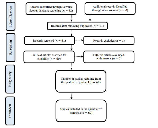
Figure 1.
Data collection flow diagram.
Citation: Rafael Gotardo, Gustavo A. Piazza, Edson Torres, Vander Kaufmann, Adilson Pinheiro. Soil Loss Vulnerability in an Agricultural Catchment in the Atlantic Forest Biome in Southern Brazil[J]. AIMS Geosciences, 2016, 2(4): 345-365. doi: 10.3934/geosci.2016.4.345
| [1] | Liudmila S. Kabir, Zhanna A. Mingaleva, Ivan D. Rakov . Technological modernization of the national economy as an indicator of green finance: Data analysis on the example of Russia. Green Finance, 2025, 7(1): 146-174. doi: 10.3934/GF.2025006 |
| [2] | Biljana Ilić, Dragica Stojanovic, Gordana Djukic . Green economy: mobilization of international capital for financing projects of renewable energy sources. Green Finance, 2019, 1(2): 94-109. doi: 10.3934/GF.2019.2.94 |
| [3] | Shahinur Rahman, Iqbal Hossain Moral, Mehedi Hassan, Gazi Shakhawat Hossain, Rumana Perveen . A systematic review of green finance in the banking industry: perspectives from a developing country. Green Finance, 2022, 4(3): 347-363. doi: 10.3934/GF.2022017 |
| [4] | Raja Elyn Maryam Raja Ezuma, Nitanan Koshy Matthew . The perspectives of stakeholders on the effectiveness of green financing schemes in Malaysia. Green Finance, 2022, 4(4): 450-473. doi: 10.3934/GF.2022022 |
| [5] | Rupsha Bhattacharyya . Green finance for energy transition, climate action and sustainable development: overview of concepts, applications, implementation and challenges. Green Finance, 2022, 4(1): 1-35. doi: 10.3934/GF.2022001 |
| [6] | Mukul Bhatnagar, Sanjay Taneja, Ercan Özen . A wave of green start-ups in India—The study of green finance as a support system for sustainable entrepreneurship. Green Finance, 2022, 4(2): 253-273. doi: 10.3934/GF.2022012 |
| [7] | Wen-Tien Tsai . Green finance for mitigating greenhouse gases and promoting renewable energy development: Case study in Taiwan. Green Finance, 2024, 6(2): 249-264. doi: 10.3934/GF.2024010 |
| [8] | Yafei Wang, Jing Liu, Xiaoran Yang, Ming Shi, Rong Ran . The mechanism of green finance's impact on enterprises' sustainable green innovation. Green Finance, 2023, 5(3): 452-478. doi: 10.3934/GF.2023018 |
| [9] | Laura Grumann, Mara Madaleno, Elisabete Vieira . The green finance dilemma: No impact without risk – a multiple case study on renewable energy investments. Green Finance, 2024, 6(3): 457-483. doi: 10.3934/GF.2024018 |
| [10] | Tao Lin, Mingyue Du, Siyu Ren . How do green bonds affect green technology innovation? Firm evidence from China. Green Finance, 2022, 4(4): 492-511. doi: 10.3934/GF.2022024 |
In the academic limelight, the concept of nation brands and brand culture, propelled by marketing specialists, has weathered challenges and debates, persistently evolving over time (Rojas-Méndez, 2016).* From a historical perspective, nation brands are associated with the rise of domestic champions. As indicated in Kalamova and Konrad (2010), this element can constitute a relevant driver for the persistence of a causal effect of nation brand values on foreign direct investment (FDI) decisions. Indeed, three central themes justify the increasing attention on nation brands:
*By underlining the role of country-of-origin as an enlightening prompt, Bilkey and Nes (1982) review country-of-origin predispositions for developing industrial assets. A comparable extension is dissected in Li and Wyer Jr (1994), Peterson and Jolibert (1995) and Verlegh and Steenkamp (1999). Maheswaran (1994) examines the effect of country-of-origin on product assessments, whereas Johansson et al. (1985) add to the discussion the impact of commonality and information about product attributes. Hong and Wyer Jr (1989) find that country-of-origin not only affects item assessments, but also animates greater considerations about other item credits. Samiee (1994) supports purchasing choice cycles inside the setting of country-of-origin and connects country-level contemplations with firm-level choices. Fan (2010) conceptualizes nation brand as a robust umbrella, which is attached to the performance of a country. With respect to proposed definitions, in an early endeavor, Kotler and Gertner (2002) characterize nation brand as the set of convictions and impressions that individuals sustain about a given spot. The picture addresses a disentanglement of countless affiliations and snippets of data associated with a spot, which are the result of mental cycles to own fundamental data. Dinnie et al. (2010) characterize nation brand as a remarkable, multi-layered mix of components that furnish the country with socially grounded separation and significance for its ideal interest groups. Fetscherin (2010) offers the vision that nation brand has a place in the public space, being complex and incorporating numerous levels, entities and learning processes. Consequently, it involves the aggregate association of partners and concerns related to a nation's whole picture by covering, among many others, political, monetary, natural and social aspects.
1. Analyze whether FDI in a host country has been driven, at least partially, by perceptions and stereotypes (Papadopoulos, 2004);
2. Confirm whether outputs of production-based economies have been dependent on international trade activities (Loo and Davies, 2006);
3. Estimate consumers' willingness to pay a premium for nation brands over private labels (Steenkamp et al., 2010).
However, as clarified in Özsomer et al. (2012), studies are neither exhausted nor limited to these traditional visions, being equally important as well to empirically evaluate whether and how nation brands are perceived by consumers (Steenkamp et al., 1999).
Beyond these traditional paradigms, this study expands its focus to brand culture, exploring its renewed relevance in the contemporary era marked by global flows of lifestyle and cultural products. The research posits compelling questions about the nature of brand meanings, the role of non-verbal cues, and the processes shaping semantic meanings in the realm of brand culture. Considering the influence of international flows, Demangeot et al. (2015) observe that the contemporaneous lifestyle and cultural products propagate worldwide independently of the development stage of each country. This stems not only from the interaction through traditional media (e.g., movies), but also from modern communication channels (e.g., vlogs). This phenomenon is changing societal patterns and fostering homogeneity on materialistic values, consumption habits, icons, and rituals (Frankenberger-Graham et al., 2015). In this sense, it is essential to obtain a greater detail about the meaning that strong nation brands and brand culture have for consumers (Steenkamp, 2019). At this level of abstraction, Batra (2019) claims the need of the following:
● Additional measures for the kind of brand meanings that can be created, as they cover a much broader domain than personality (e.g., refinement and vulgarity, delicacy and strength, sensuality and security, and nurturance and confidence);
● Analyzing other types of stimuli, namely those created by non-verbal and facial cues (e.g., colors, logos, music, and styles) and sensory elements (e.g., smell, taste, and touch) to identify how they facilitate the transfer of a brand's cultural meaning;
● Better understanding the nature of processes that create semantic meanings, which are likely different from those that provide pleasure to consumers.
In a reflection about the promotion of destination and place branding, Hewett et al. (2022) highlight the need to accommodate a supranational conceptualization of nation brand to effectively transcend any existing geographical boundary between countries. Özsomer (2012) suggests that cross-national learning in the context of city branding should overcome organizational challenges, which requires target groups and their articulation with sectoral marketing practices, establishing urban narratives about the need to represent the city's heritage, using novel communication actions and channels, and customizing a collaborative model for city branding.
Equally impressive as well is the seminal contribution of Belk (1984), which proposes three measures (i.e., possessiveness, non-generosity, and envy) to quantify materialistic traits. However, leveraging a brand that pretends to stimulate consumption and/or materialism currently requires deeper strategic actions, which must be differentiated from standard digital-based initiatives. As extrapolated from Gielens and Steenkamp (2019), the challenge is to make wise choices within the digital environment, which requires a minimum threshold of critical ability to express the materialistic story and ensure the brand's adaptability to a wide range of different communication channels.
There is also a vast strand of research supporting the argument that universities act as a promotion flag for some countries, which establishes the notion of scientific brand (Caffrey and Isaacs, 1971; Benneworth and Charles, 2005; Wakkee et al., 2019). In addition, the agreement signed by 193 countries on 17 United Nations Sustainable Development Goals (UN-SDG) in September 2015 was a key step to boost the proliferation of green brand economies, whose principle is to defend the environmental cause and ensure the primacy of sustainable development over economic growth (Gössling and Humpe, 2020). Moreover, despite the lack of consensus, nation brand studies have been warning about the emergence of nationalist ideologies (Anholt, 2002; Aronczyk, 2008; Bulmer and Buchanan-Oliver, 2010; Volcic and Andrejevic, 2011). All these sources of observed heterogeneity in the literature focused on nation brands and brand culture lead us to formulate three research questions, which constitute the motivation behind this work:
1. RQ1: How is the evolution of studies in this literature characterized?
2. RQ2: How many and which kind of clusters exist to represent the possible set of marketing strategies for a country to become a brand with global notoriety?
3. RQ3: Which future trends and associations can be established between the emergent field of green finance and the existing literature on nation brands and brand culture?
Embarking on a systematic bibliometric analysis, this study aims to scrutinize nuanced strategies that nations employ to secure global prominence. Traditionally, bibliometric analyses have been perceived as instruments for surveying the historical contours of a specific research field. However, this study breaks free from this mold, championing a visionary approach that goes beyond the confines of traditional boundaries. In the vast landscape of bibliometric analyses, a paradigm shift is underway, challenging the conventional view that confines such analyses to a retrospective literature review. This study boldly embraces a broader perspective, asserting that bibliometric analyses are not just tools for navigating the troves of existing knowledge; rather, they serve as beacons illuminating uncharted territories of future research. Central to this transformative stance is the application of bibliometric analysis to the intricate realms of nation brands and brand culture, aiming not only to decipher their evolution but to unlock novel pathways for the field of green finance. Therefore, by scrutinizing 60 articles from 1992 to 2021, the analysis discerns not just the trajectories of nation brands but envisages their intersection with the burgeoning field of green finance. At the heart of this paradigm lies a groundbreaking objective, which is to identify niche opportunities that seamlessly bridge the realm of nation brands, brand culture, and the evolving landscape of green finance.
This research delves into the multifaceted world of nation brands and brand culture, propelled by two overarching questions: How can a country become a world-renowned brand? How does this achievement affect the field of green finance? By integrating both contexts, this study navigates the landscape of nation brand evolution, employing an innovative combination of latent Dirichlet allocation (LDA) with a multinomial and unordered discrete choice analysis (DCA). In addressing these pivotal research questions with appropriate methods, this study lays the foundation for a systematic review, offering insights into the evolution of studies on nation brands and brand culture, unveiling clusters of marketing strategies, and discerning future trends and associations of country branding with the field of green finance.
The significance of this approach is manifold. First, it challenges the siloed nature of academic inquiry, heralding an era where the interconnectivity of seemingly disparate fields is not just acknowledged but actively explored. Nation brands and brand culture, typically nestled within the folds of international marketing, emerge as catalysts for sparking innovation and transformation in green finance. Second, the study identifies six distinctive marketing strategies for countries aspiring to global notoriety, namely joint integration of country-of-origin and city brands, consumption brand, materialistic brand, green brand, ideological brand, and scientific brand. Three central themes, delving into perceptions, international trade dependencies, and consumer preferences, further underscore the growing significance of nation brands and brand culture in a globalized landscape. Additionally, the study identifies the supranational conceptualization of nation brand and brand culture as a pivotal action to leverage the field of green finance, transcending geographical boundaries. Consequently, the interconnectedness of city branding, materialistic traits, scientific branding, and the emergent themes of green nation brands and green brand culture are meticulously examined. Third, the research underscores the temporal evolution of environmental branding strategies, gaining preponderance globally after 2015. In tandem, the emergence of ideological branding as a recent trend echoes a conscientious shift towards enhancing national identity systems. The intersection of these trends with green finance beckons a compelling exploration of eco-centric investment strategies and the alignment of financial practices with sustainable national values. These strategies, when viewed through the lens of green finance, unveil unprecedented opportunities for sustainable investments, eco-friendly initiatives, and the integration of environmental considerations into financial frameworks. Fourth, our empirical assessment underscores the imperative for a multidisciplinary approach in crafting nation brands, revealing that divergent strategies need not be mutually exclusive. Strategic guidance for nations is illuminated, emphasizing the importance of assuming a Stackelberg leadership role to generate added value.
Notably, these insights collectively underscore the transformative potential of bibliometric analysis in decoding the evolution of nation brands and brand culture to the benefit of alternative research fields, such as green finance. The study culminates in a thought-provoking reflection on the increasing notoriety of ideological branding and its implications for the sustainability of democratic regimes, green political parties and their relationship with green finance, providing a compelling platform for future research endeavors in this dynamic field. In conclusion, this study pioneers a transformative vision, leveraging bibliometric analysis not just as a retrospective tool but as a forward-looking compass. By bridging the realms of nation brands, brand culture, and green finance, it unravels a tapestry of niche opportunities, urging researchers and practitioners to explore the uncharted territories where environmental sustainability and financial acumen converge. This innovative approach holds promise for shaping a sustainable future where academic exploration transcends disciplinary boundaries, propelling research and practice towards a holistic understanding of the complex interplay between country branding, brand culture, and green finance.
Bibliometric studies have gained prominence across various research fields, thanks to their contribution to promoting, organizing, and disseminating scientific knowledge (Ribeiro and Cirani, 2013). This study adopts a hybrid approach, seamlessly integrating bibliographic and bibliometric techniques (Silva and Teixeira, 2009). Recognizing the enhanced efficiency that well-defined protocols bring to systematic literature reviews, the hybrid approach is structured into two distinct stages: a qualitative protocol and a quantitative procedure.
The qualitative protocol necessitates the development of a clear research strategy to acquire representative studies. While there is no universally prescribed rule for extracting relevant articles, it is advisable to adopt criteria established by previous bibliometric studies. This not only ensures objectivity and transparency but also mitigates the risk of criticism regarding misinterpretation and judgment (Roztocki and Weistroffer, 2008). Nevertheless, Boell and Cecez-Kecmanovic (2015) argue that bias linked to subjectivity in systematic literature reviews is unlikely to be entirely eradicated. They emphasize the crucial need to maintain objectivity. Based on these premises, the qualitative protocol comprises four steps:
● Specification of databases;
● Definition of search terms;
● Establishment of inclusion and exclusion criteria with internal and external validation; and
● Clarification of the final selected sample.
Conducting a systematic literature review demands meticulous, transparent, and reproducible research to identify a comprehensive array of relevant studies (Falagas et al., 2008). While various sources can be consulted, bibliographic databases stand out as the primary choice due to their extensive journal coverage and ease of access (Adriaanse and Rensleigh, 2013). Consistent with the approach outlined by Abramo et al. (2011), the search for pertinent articles was executed by collecting data from SciVerse Scopus.
Not all databases feature controlled language. The utilization of Boolean operators, represented by AND, OR, and NOT, enables the formulation of term combinations. Given the challenge associated with identifying quality content in verification processes (Norris and Oppenheim, 2007), this step establishes the set of relevant studies through the adoption of the following search code:†
†(TITLE-ABS-KEY(Nation Brands) AND TITLE-ABS-KEY(Brand Culture)) AND (LIMIT-TO (PUBSTAGE, "final")) AND (LIMIT-TO (DOCTYPE, "ar")) AND (LIMIT-TO (LANGUAGE, "English")) AND (LIMIT-TO (SRCTYPE, "j")) AND (LIMIT-TO (SUBJAREA, "BUSI"))
In alignment with the methodology proposed by Chappin and Ligtvoet (2014), the search encompasses three dimensions – title, abstract, and keywords – aiming to minimize the occurrence of false positives. The terms nation brand and brand culture were selected to ensure the comprehensive capture of core contributions. The inclusion of these terms was carefully considered to discourage irrelevant information and prevent redundancy (D'Angelo et al., 2011). Cohen (1992) and Lewison (1998) assert that such an approach helps alleviate the presence of false negatives. It is worth noting that the consulted databases employ stemming, automatically accounting for term variants.
The initial search is limited to finalized articles, excluding any studies classified as comments, conference papers, reviews, conference reviews, corrigenda, books, book chapters, notes, editorials, short surveys, or letters. Furthermore, the search is narrowed down to the field of business, management, and accounting. Only finalized articles written in English and published in academic journals are considered, aligning with the criteria outlined by Pato and Teixeira (2016). To ensure a robust and unbiased selection, we employ additional qualitative criteria to test the data extraction model and assess study quality. A visual inspection of the title, abstract, and keywords of relevant studies is conducted, and in some cases, authors are contacted to re-evaluate eligibility criteria. The final decision regarding the inclusion or exclusion of core contributions is made prior to data extraction, ensuring procedural consistency.
As confirmed in Figure 1, which presents the data collection flow diagram following Demir et al. (2024a, b), the final sample comprises 60 articles published between 1992 and 2021. It is important to emphasize that the time period is endogenously determined by the algorithm associated with the database. This approach implies no imposition of any starting year for the sample, thereby avoiding biased estimations resulting from self-selection and subjective judgment. It should be noted that any qualitative protocol is susceptible to weaknesses, such as the potential inclusion of alternative studies, and limitations, such as a temporal gap between search development and publication date. Consequently, results from the subsequent quantitative analysis should be approached with caution (Osareh, 1996). The extracted data underwent thorough scrutiny to derive valid and logical conclusions. The synthesis phase involved collecting, combining, and summarizing the findings of individual studies included in the systematic literature review, employing formal statistical techniques (e.g., meta-analysis) and qualitative procedures (e.g., narrative approach). The final summary integrates the strength of empirical outcomes, examines the consistency of observed effects across studies, and elucidates potential reasons for any discrepancies. Following the individual analysis of all studies, we proceed to the quantitative procedure.
This stage includes treating data, evaluating evidence, and disseminating outcomes through a quantitative procedure, which is organized as follows:
● Assessment of relevant studies by year and journal;
● Clarification of the most cited work and main contributors;
● Co-occurrence map analysis of representative terms of the research field under scrutiny;
● Adoption of LDA and DCA in multinomial and unordered form to classify possible marketing strategies for a country to become a world-renowned brand.
We commence by illustrating the distribution of studies by year and journal. The time series analysis delves into the dynamics of scientific publications, examining variations over time and assessing their substitutability and complementarity concerning a broader control group of studies captured by the term national brands.‡ The quantitative analysis also identifies pertinent academic journals, highlights the most cited articles, and pinpoints the main contributors within the scope of this research field.
‡The search code is described as follows:
TITLE-ABS-KEY (national AND brands) AND (LIMIT-TO (PUBSTAGE, "final")) AND (LIMIT-TO (PUBYEAR, 2021) OR LIMIT-TO (PUBYEAR, 2020) OR LIMIT-TO (PUBYEAR, 2019) OR LIMIT-TO (PUBYEAR, 2018) OR LIMIT-TO (PUBYEAR, 2017) OR LIMIT-TO (PUBYEAR, 2016) OR LIMIT-TO (PUBYEAR, 2015) OR LIMIT-TO (PUBYEAR, 2014) OR LIMIT-TO (PUBYEAR, 2013) OR LIMIT-TO (PUBYEAR, 2012) OR LIMIT-TO (PUBYEAR, 2011) OR LIMIT-TO (PUBYEAR, 2010) OR LIMIT-TO (PUBYEAR, 2009) OR LIMIT-TO (PUBYEAR, 2008) OR LIMIT-TO (PUBYEAR, 2007) OR LIMIT-TO (PUBYEAR, 2006) OR LIMIT-TO (PUBYEAR, 2005) OR LIMIT-TO (PUBYEAR, 2004) OR LIMIT-TO (PUBYEAR, 2003) OR LIMIT-TO (PUBYEAR, 2002) OR LIMIT-TO (PUBYEAR, 2001) OR LIMIT-TO (PUBYEAR, 2000) OR LIMIT-TO (PUBYEAR, 1999) OR LIMIT-TO (PUBYEAR, 1998) OR LIMIT-TO (PUBYEAR, 1997) OR LIMIT-TO (PUBYEAR, 1996) OR LIMIT-TO (PUBYEAR, 1995) OR LIMIT-TO (PUBYEAR, 1994) OR LIMIT-TO (PUBYEAR, 1993) OR LIMIT-TO (PUBYEAR, 1992)) AND (LIMIT-TO (DOCTYPE, "ar")) AND (LIMIT-TO (SUBJAREA, "BUSI")) AND (LIMIT-TO (LANGUAGE, "English")).
The content of selected studies undergoes classification through a term co-occurrence map analysis conducted using VOSviewer 1.6.8 (Eck and Waltman, 2009, 2010; Waltman et al., 2010). This operation segments the diversity of content among the selected articles and ensures the identification of statistically significant relationships (Khasseh et al., 2017). The mining routine operates on the existing text data in the title, abstract, and keywords of relevant articles, considering either global or local centrality measures that capture the strength of links between selected noun phrases, referred to as terms (Gan and Wang, 2015).
We adhere to the methodology proposed by Eck and Waltman (2011), who developed a technique for selecting the most relevant terms. First, the distribution of second-order co-occurrences for each noun phrase is analytically determined. Subsequently, each individual distribution is compared against the overall distribution of co-occurrences. The larger the difference between both distributions, the higher the expected relevance of a term. The difference between individual and overall distributions is formally measured by the Kullback-Leibler distance or relative entropy. For discrete probability distributions P and Q defined on the same probability space χ, the relative entropy from Q to P is given by
| DKL(P | Q)=∑x∈χP(x)log[P(x)Q(x)] |
or equivalently
| DKL(P | Q)=−∑x∈χP(x)log[Q(x)P(x)] |
which corresponds to the expectation of a logarithmic difference between probabilities P and Q. Relative entropy is defined only if Q(x)=0 implies P(x)=0 (i.e., absolute continuity) for all x∈χ. Whenever P(x) is zero, the contribution of the corresponding term is null because
| limx→0+xlog(x)=0. |
According to Eck and Waltman (2011), terms with low relevance (i.e., noun phrases with a general meaning) exhibit a more or less equal distribution of their second-order co-occurrences, while terms with high relevance (i.e., noun phrases with a specific meaning) display a distribution of their second-order co-occurrences significantly biased towards certain terms. Consequently, a co-occurrence network map assumes that terms with high relevance cluster together, where each cluster can be interpreted as a topic of interest within the research domain under scrutiny. This choice is justified by the premise that existing terms in the title, abstract, and keywords of relevant articles are sufficient to describe the intellectual core of a given research field, both in relative terms and over time (Zong et al., 2013). We specifically focus on betweenness centrality (BC) to measure the interdisciplinarity of relevant articles. As clarified in De Nooy (2011), the BC of a vertex k is equal to the proportion of all geodesics between pairs (gij) of vertices that include this vertex (gijk). Formally
| BCk=∑i∑jgijkgij, i≠j≠k. |
According to Freeman (1977), the primary advantage of adopting social network analysis lies in its reliability, attributed not only to the diverse centrality measures that can be implemented but also to its flexibility in split sample analyses, making it perfectly adaptive to a diversified set of statistical criteria. However, a notable disadvantage is the challenge of interpreting the final outcomes. Following the identification of final clusters, the analysis is complemented by intra- and inter-cluster diversity measures.
Intra-cluster diversity. It evaluates the extent and degree to which the internal knowledge base is diverse for a given cluster through measures of diversity, evenness, and richness. The concept of diversity, historically rooted in information theory, finds application in various research domains such as ecology. In ecology, a sample of species is likened to a message and the number of individual organisms corresponds to pieces of information (Magurran and McGill, 2011). In the context of this study, a sample of species pertains to terms within a given cluster, while the number of individual organisms represents the number of links associated with these terms. A general measure of information for infinitely large sets of terms is the Renyi entropy of order α. The focus of this study centers on the limit value as α→1 (Hill, 1973), wherein the discrete Shannon-Wiener diversity index of each cluster simplifies to
| H′=Ri=−∑ipilnpi, |
where pi represents the proportion or relative weight of the link of term i. According to Margalef (1972) and May (1979), the index value usually satisfies 1≤H′≤4.5 and surpassing the ceiling is rare. Following the methodology of Appio et al. (2014) and Appio et al. (2016), two additional measures are considered to assess the degree of intra-cluster diversity: richness (S), representing the total number of terms identified within a given cluster; and evenness (E), the ratio of observed diversity (H′) relative to maximum diversity (Hmax). Evenness corresponds to
| E=H′Hmax. |
In turn, maximum diversity is given by
| Hmax=lnS. |
The index satisfies 0≤E≤1, where the floor (ceiling) represents a situation where species are asymmetrically (equally) abundant, respectively. To compute these indices, we gather all representative terms of each cluster, standardize their names, and determine their relative abundance (Pielou, 1969).
Inter-cluster diversity. It assesses whether a given cluster is more diverse compared to other groups by performing the t-test proposed by Hutcheson (1970), which examines diversity differences between clusters. The null hypothesis posits that two Shannon diversity indices originate from two communities with equal species diversity (Magurran, 1988). Therefore, not rejecting the null hypothesis implies the persistence of two homogeneous clusters or, similarly, the absence of inter-cluster diversity, indicating that both groups share a common knowledge base. In contrast, rejecting the null hypothesis implies that two clusters have heterogeneous knowledge bases, signifying that both groups have a different conceptual nature.
The entire process comprises three steps:
1. Development of preliminary tasks;
2. Identification of explanatory variables to classify the target;
3. Clustering articles into categories, whose optimal number is endogenously determined by content analysis that has learned sequential patterns from the text data. After defining the target, evaluate the likelihood of developing research for a given category.
While the second step is executed through an LDA model, the third step employs a DCA in multinomial and unordered form.
Preliminary tasks. Preliminary tasks encompass importing input data (i.e., title, abstract, and keywords of articles), removing unnecessary punctuation, converting labels to the categorical type, visualizing the distribution of classes in histograms and obtaining frequency counts, and identifying infrequent categories (i.e., those with a low number of observations and removing them; as a rule of thumb, all terms with a frequency below 10 were eliminated).
Latent Dirichlet allocation. Seminally developed by Blei et al. (2003), LDA is a popular machine learning model that clusters text data into a predefined number of classes. In this model, each document is represented as a probability distribution over topics, and each topic internalizes a probability distribution over words. Therefore, LDA provides a clear and objective method for analyzing the content of unclassified text data through two steps:
1. The probabilistic model, which describes text data as a likelihood function;
2. An approximate inference algorithm, given that maximizing such a likelihood function is computationally unfeasible.
Following the approach of Schwarz (2018), it is mathematically assumed that each text data d of D articles is described as a probabilistic mixture of T topics. These probabilities are contained in a topic vector θd of length T. Consequently, the output of LDA is a D×T matrix θ containing P(t|d), which represents the probability of text data d belonging to topic t.
| θ=[θ1⋮θD]=[P(t1|d1)...P(tT|d1)⋮⋱⋮P(t1|dD)...P(tT|dD)] |
Each topic t∈T is characterized by a probabilistic distribution over the set of words of size V. Consequently, a topic describes the likelihood of observing a word conditional on that topic. The word-probability vectors of each topic are encompassed in a matrix ϕ of dimension V×T
| ϕ=(ϕ1,...,ϕT)=[P(w1|t1)...P(w1|tT)⋮⋱⋮P(wV|t1)...P(wV|tT)] |
Probabilities P(wv|tt) indicate how likely it is to observe word v given topic t. Therefore, the ϕt vectors enable the assessment of the content of each topic since LDA does not provide additional topic labels. With parameters θ and ϕ, the probabilistic model posits that text data are generated by the following process:
1. Draw a word-probability distribution ϕ∼Dir(β);
2. For each article d:
● Draw topic proportions θd∼Dir(α);
● Considering the set of Nd words, draw a topic assignment zd,n∼Mult(θd) for each word wd in d, and a word wd,n from p(wd,n|zd,n,ϕ).
Both α and β serve as essential hyperparameters for the Gibbs sampling process. The LDA classification relies on determining the optimal topic assignment zd,n for each word in each article and optimal word probabilities ϕ for each topic that maximizes this likelihood. This necessitates summing over all possible topic assignments for all words in the set of articles. Given that this task is computationally unfeasible, alternative methods to approximate the likelihood function have been developed.
§ Given the probabilistic model, the overall likelihood with respect to parameters is expressed as
| D∏d=1P(θd,α){Nd∏n=1 ∑zd,nP(zd,n,θd)P(wd,n,ϕ)} |
where P(θd|α) is the likelihood of observing the topic distribution of θd in article d conditional on α, P(zd,n|θd) is the likelihood of topic assignment zd,n of word n in article d conditional on the topic distribution of the article, and P(wd,n|zd,n,ϕ) is the probability to observe a specific word conditional on the topic assignment of the word and word probabilities of the given topic contained in ϕ. We obtain the likelihood of observing a given word in each article by calculating the sum over all possible topic assignments (∑z), the product over all Nd words in a document (∏Ndn=1), and the product over all articles in their set (∏Dd=1).
This study employs Gibbs sampling, a Markov chain Monte Carlo algorithm based on repeatedly drawing new samples conditional on the existing data. The process begins by converting input data into numerical sequences of word tokens, achieved through iteratively updating the topic assignment of words conditional on the topic assignments of all other words. Gibbs sampling operates as a Bayesian technique, necessitating priors for the hyperparameters α and β, which should fall within the unit interval.¶ Afterwards, word tokens are randomly assigned to one of the T topics with equal probability, while the algorithm samples new topic assignments for each word token. The probability of a word token being assigned to topic t based on the probabilistic model corresponds to||
¶The prior for α is normally based on the number of topics T, while the prior for β depends on the amount of words. According to Griffiths and Steyvers (2004), α=50/T and β=0.1.
||The Gibbs sampler uses the topic assignment of all tokens to obtain approximate values for P(wd,n|zd,n=t,ϕ) and P(zd,n=t). P(wd,n|zd,n=t,ϕ) is given by the number of words identical to wd,n assigned to topic t divided by the total number of words assigned to that topic. P(zd,n=t) is given by the fraction of words in the article assigned to topic t plus the prior for α.
| P(zd,n=t|wd,n,ϕ)∝P(wd,n|zd,n=t|ϕ)×P(zd,n=t). |
Discrete choice analysis. Initially developed by McFadden (1974), DCA is a classification method to assess the probability that a certain observation i falls into one of the m categories that characterize the target yi. A multinomial density for a single observation is given by f(yi)=m∏j=1pyjij, where the probability that observation i belongs to category j corresponds to pij=P[yi=j|X]=Fj(Xβ), with i={1,...,n}, j={1,...,m}. A multiple linear regression model in matrix notation is given by Y=Xβ+u, where Y is the vector (n×1) that represents the dependent variable or target, X corresponds to the matrix (n×k) of input components 1, X2i, X3i, ..., Xki, β is the vector (k×1) of coefficients, parameters or weights associated with the independent term and regressors, and u is the vector (n×1) of disturbance terms. In any DCA, the functional form of Fj(⋅) should be selected. Each pij lies between 0 and 1, so that their sum over j is equal to 1. An exception occurs with the linear probability model because the respective binomial distribution implies Fj(Xβ)=Xβ such that pij=P[yi=j|X]=Xβ. Consequently, the most common choice for the functional form of F(⋅) is the logistic distribution (reduced normal distribution) representative of a logit (probit) model, respectively.** From a theoretical point of view, McFadden (1974) confirms that the choice between logit and probit models depends on the type of characteristics sustained by the dependent variable, whereas McFadden et al. (1977) detail that, if the dependent variable can be directly observed, then a logit model is expected to be the optimal choice. Hahn and Soyer (2005) find evidence that the logit specification provides a better goodness-of-fit with extreme values in multinomial response settings. Conversely, the goodness-of-fit in moderate size datasets is improved by selecting the probit specification with random effects. Despite these normative postulates, this study follows objective criteria to determine the optimal model, which should exhibit the lowest Akaike information criterion (AIC) or Bayesian Information criterion (BIC) and the highest log-pseudolikelihood.
**In the probit model, F(⋅) is the normal distribution function Φ(ui)=ui∫−∞1√2πe−12t2dt, whose probability density function is ϕ(ui)=dΦ(ui)dui=1√2πe−12u2i. In the logit model, F(⋅) corresponds to Λ(ui)=11+e−ui, which is the distribution function of a logistic variable with zero mean and variance π2/3. The respective probability density function is λ(ui)=dΛ(ui)dui=e−ui(1+e−ui)2. It is easily verifiable that the equality λ(ui)=Λ(ui)[1−Λ(ui)] holds.
In light of the multinomial and unordered response model applied to this study, the probability that article i belongs to cluster j is given by††
†† The target is classified as follows: cluster 1 corresponds to consumption branding, cluster 2 corresponds to ideological branding, cluster 3 corresponds to environmental branding, cluster 4 corresponds to country-of-origin/city branding, cluster 5 corresponds to university branding and cluster 6 corresponds to materialism branding. The choice of the category to which each article belongs, Articlei=j|X, is exogenous and independent from the set of explanatory variables to avoid endogeneity problems, with i={Article 1,...,Article 60},j={Cluster 1,...,Cluster 6}.
| pij=P[Articlei=j|X]=Fj(Xβ) |
with i={Article 1,...,Article 60} and j={Cluster 1,...,Cluster 6}. The set of explanatory variables used for the DCA is given by X=[Topic 1,...,Topic 6], whose numeric values result from the application of LDA clarified in the Prediction and classification of future research trends subsection.
Although a certain classification is endogenously imposed on each article, it is not considered in isolation. The content of each article is influenced by information related to other strands of the literature according to X. Intuitively, this innovative meta-analysis captures the complementarity between the different strategies used to define nation brand and brand culture when writing a scientific article. The deterministic component Fj(Xβ) must be normalized to ensure the estimation of 5 coefficients. Therefore, model identification requires setting βj to zero for one category, assumed to be the base category. Then, the estimated coefficient of category j has a straightforward qualitative interpretation: compared to the base category, an increase in a continuous explanatory variable from the set of inputs X makes adherence to category j more or less likely, depending on the sign exhibited by the respective estimated coefficient. Additionally, the probability that article i belongs to category j can be rearranged as follows
| pij=pr[Articlei=j|X]=exp(Xβj)∑6k=1exp(Xβk) |
such that, for each regressor, the marginal effect of a change on the probability of belonging to alternative j is given by
| ∂pij∂Topic t=pij(βk−βl) |
with k≠l and t={1,...,6}. There will be 6 marginal effects corresponding to 6 predicted probabilities. Their sum over the different categories that define the target is equal to zero because predicted probabilities sum to 1. Their quantitative interpretation is straightforward: an increase in a continuous explanatory variable from the set of inputs X either increases or decreases the probability of belonging to category j by the marginal effect − either average, at the mean or for specific values taken by each component of X − expressed in percentage terms. Finally, it should be clarified that:
● Statistical tests for individual and joint significance are performed;
● All regressors are alternative-invariant (i.e., they vary over article i, but do not vary over category j, with i={Article 1,...,Article 60} and j={Cluster 1,...,Cluster 6});
● The satisfaction of the independence from irrelevant alternatives (IIA) assumption is verified through the Suest-based Hausman-McFadden test, whose null hypothesis is that the odds ratio of two categories is independent from other alternatives.
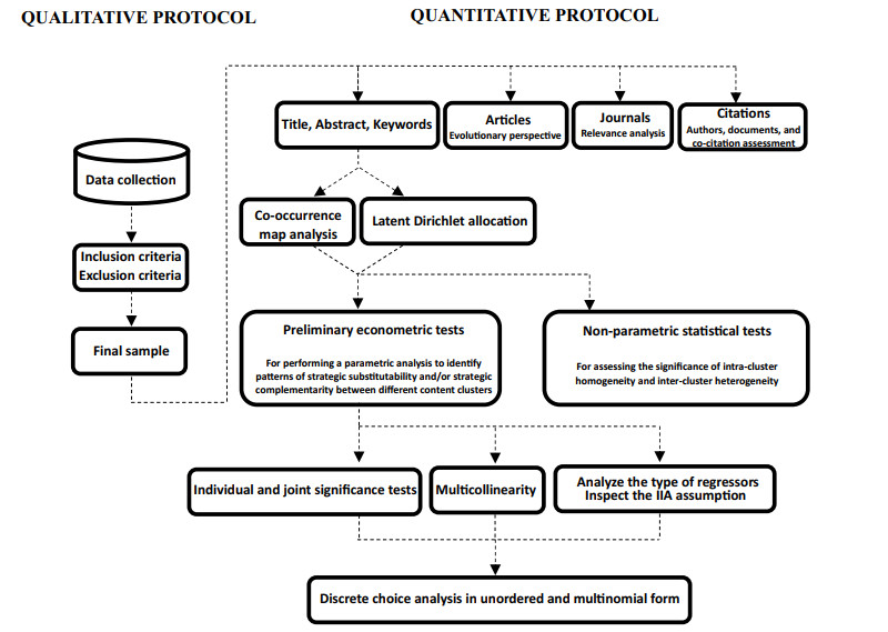
Similar to recent bibliometric studies applied to alternative research domains (Marino-Romero et al., 2023; Aguilar-Moreno et al., 2024), the methodological pipeline is summarized in Figure 2. Table A1 in Appendix provides a compilation of previous systematic literature reviews and bibliometric analyses related to the topic under scrutiny.
Observations are grouped into classes, the number of which should be determined endogenously. Given that each class has a specific width, known as the class interval, we need to satisfy the relation between the class interval and the number of classes
| xi≥maxyi−minyik |
where xi is the class interval, k represents the number of classes and elements of the numerator correspond to the maximum and minimum value of the target.‡‡
‡‡Knowing that we define 10 classes to segment the time period [1992, 2021], it follows that
| xi≥2021−199210⇔xi≥2.9 |
Therefore, the natural number immediately above 2.9 was used to define the interval class.
Figure 3a shows that the evolution of scientific articles focused on nation brand and brand culture is non-monotonic over time, thus allowing to provide a first clear answer to RQ1. After two peridos without observing any output, there is an increasing number of published articles until the period [2010, 2012]. Thereafter, there is a reduction of published articles in the following two periods, followed by another rise of scientific production in the period [2019, 2021]. When Figures 3a – 3b are simultaneously visualized, a remarkable pattern is the persistence of a similar behavior between representative functions of the absolute and relative number of published studies focused on nation brand and brand culture. The downward adjustment of the relative weight of published articles is particularly pronounced in the period [1992, 1994] and between 2013 and 2018. While the former case materializes the presence of a sleeping beauty as defined in Teixeira et al. (2017), the later one may reflect a circumstantial reduction of interest on this scientific domain. Nothwithstanding, there is a rise in the proportion of nation brand and brand culture articles over the total universe of national brand articles in two periods: between 2001 and 2012, and after 2018.
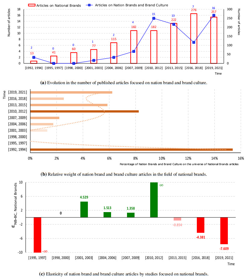
Although interesting, the previous result is insufficient to provide valuable information about the strategic interaction between both research fields. In order to infer whether a given period is characterized by either complementarity or substitutability when confronting nation brand and brand culture articles against the scientific production covering national brands, one needs to apply the concept of elasticity. From a theoretical point of view:
● A positive (negative) elasticity, materialized by the green (red) color in Figure 3c, reflects a strategic complementarity (substitutability) between treatment and control groups, respectively;
● An elasticity greater (lower) than 1, marked by the dark (light) tint in Figure 3c, reflects an elastic (inelastic) relation between both strands of research.§§
§§That is, a strong or above 1% (weak or below 1%) variability of published articles focused on nation brand and brand culture for a 1% change in the number of published articles focused on national brands, respectively.
One should start by emphasizing that Figure 3a confronts the evolution of published articles focused on nation brand and brand culture against the evolution of studies focused on the broader field of national brands (e.g., while the former research domain restricts the search for brands at the country level, the later one also accommodates corporate brands). Results indicate that the cumulative sum of 60 core contributions related to nation brand and brand culture only represents 4.2% of the total number of published studies concerned with national brands between 1992 and 2021 (n= 1,425), which suggests that there is some degree of freedom for additional contributions focused on the niche field under scrutiny.
Figure 3c highlights that, from the period [1992, 1994] to the period [1995, 1997], the number of nation brand and brand culture (national brands) published articles decreases (increases) to 0 (41), respectively. As such, the elasticity of nation brand and brand culture articles by published studies focused on national brands converges to −∞ in the period [1995, 1997]. Thereafter, the period [1998, 2000] confirms that published articles on nation brand and brand culture (national brands) remain null (increase to 60), respectively. Consequently, the respective elasticity takes the null value, which confirms that nation brand and brand culture studies materialize a sleeping beauty niche during this time period. A positive and elastic relationship between both research fields is identified after the period [1998, 2000]. In fact, their relation becomes perfectly elastic in the period [2010, 2012] given that the number of published articles focused on nation brand and brand culture increases (national brands remains stable) compared to the previous triennium, respectively. This result reinforces that between 2001 and 2012 lies the period of greatest scientific expression of nation brand and brand culture. Thenceforth, a permanent and negative elasticity is observed, which reflects a reduction of the relative importance of nation brand and brand culture on national brands between 2013 and 2021. This reduction is stronger as time converges to 2021 given that elasticity values are increasingly negative. In summary:
● There is strategic substitutability between national brands and the nation brand−brand culture pair before the sleeping beauty period [1998, 2000] and after 2013;
● There is strategic complementarity between national brands and the nation brand−brand culture pair after the sleeping beauty period [1998, 2000] and until 2012; and
● The relation between both research domains is predominantly elastic.
The total number of articles focused on nation brand and brand culture is distributed over a set of 44 academic journals. Figure 4a details the Top–5 ranking list, which shows that the most relevant outlets for this niche literature are:
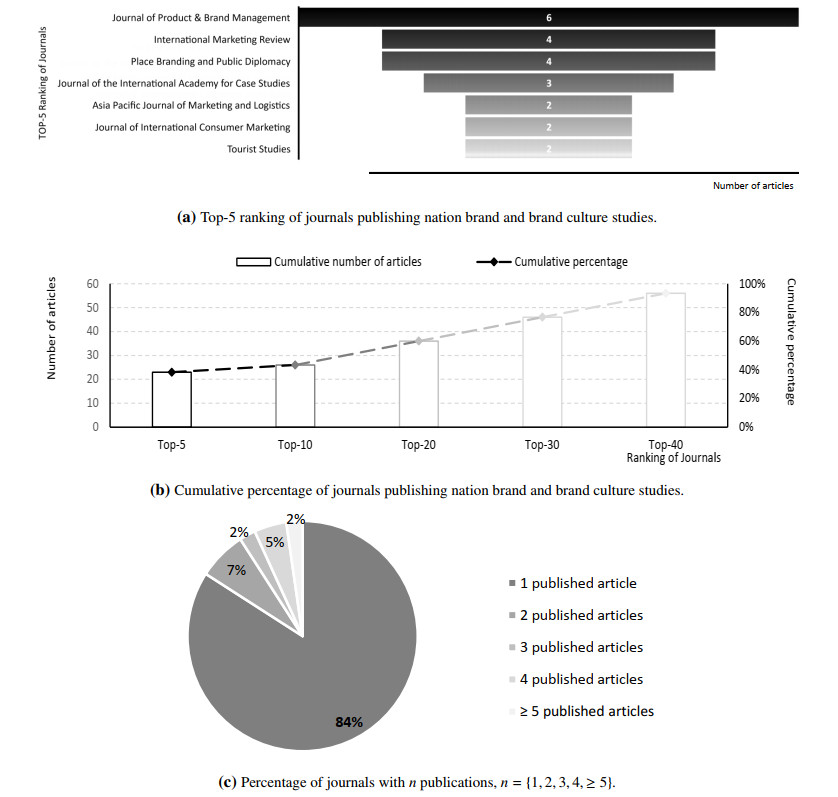
1. Journal of Product & Brand Management, founded in 1992 and currently with six published articles (Q1 in Management of Technology and Innovation; 2019 IF: 1.832);
2. International Marketing Review, founded in 1983 and currently with four published articles (Q1 in Business and International Management; 2019 IF: 4.198);
3. Place Branding and Public Diplomacy, founded in 2004 and currently with four published articles (Q3 in Marketing; 2019 IF: N/A; ¶¶
¶¶Because it is not indexed in Clarivate Analytics.
4. Journal of the International Academy for Case Studies, founded in 1995 and holding three published articles (Q4 in Business and International Management; 2019 IF: N/A);
5. The fifth place is co-shared by three academic journals that contemplate two articles each, namely: Asia Pacific Journal of Marketing and Logistics, which was founded in 1993 (Q2 in Business and International Management; 2019 IF: 2.511); Journal of International Consumer Marketing, which was founded in 1988 (Q2 in Management Information Systems; 2019 IF: N/A) and Tourist Studies, which was founded in 2001 (Q2 in Tourism, Leisure and Hospitality Management; 2019 IF: 1.391).
Journals within the Top–5 were established between 1983 and 2004, indicating a relatively low level of maturity. Additionally, they tend to have a moderate impact factor, reflecting an emerging level of recognition. The cumulative percentage of published articles in the Top–10 (Top–20) [Top–30] ranking of journals is 43% (60%) [77%], respectively. The 50th percentile of published articles falls between Top–30 and Top–40 outlets (Figure 4b). While 84% of journals published a single study, only 2% contain at least five articles focused on the topic under scrutiny (Figure 4c).
Overall, these findings suggest that scientific production focused on this niche literature can benefit from increasing returns to scale. They also indicate that journals with a moderate reputation are open to publishing nation brand and brand culture studies and publication activity is likely to grow and sustain strong recognition in the future. Moreover, a spillover effect arises from the accommodation of scientific production by high-quality outlets, emphasizing the substantial potential of nation brand and brand culture as a research field—a point not to be overlooked by new scholars.
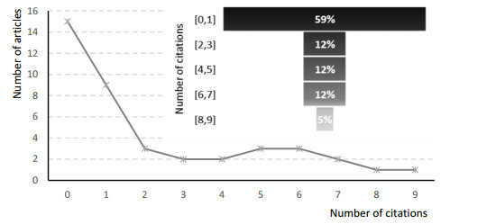
Table A2 in Appendix compiles the list of published articles with 10 or more citations, which corresponds to 31.7% of the sample. These were predominantly published in 2010 and 2013, which suggests that the most cited studies are characterized by a small within variation. The main outlet for knowledge dissemination is the Journal of Product & Brand Management (15.8%). For the subsample of published articles that were cited less than 10 times, 59% has one or zero citations (Figure 5). This result indicates that research focused on nation brand and brand culture is concentrated in a limited number of studies.
Three types of citation networks are presented, which are based on:
● Citation analysis applied to documents, where the relatedness of nation brand and brand culture studies is determined by the number of times they cite each other;
● Citation analysis applied to authors, which is similar to the previous exercise but with the difference that it focuses on authors; and
● Co-citation analysis, where the relatedness of authors is determined by the number of times studies are cited together.
Results of the citation analysis applied to documents are elucidated in Figure 6. These help identify the preponderance of Foscht et al. (2008), which is complemented and interconnected with four studies respectively developed by Mooij (2003), Wallström et al. (2010), Maciel et al. (2013) and Alserhan et al. (2015). Results of the citation analysis applied to authors are clarified in Figure 8, revealing that this niche literature is predominantly influenced by B. Swooboda, I. Sinha, T. Foscht, D. Morschett, and C. Maloles.
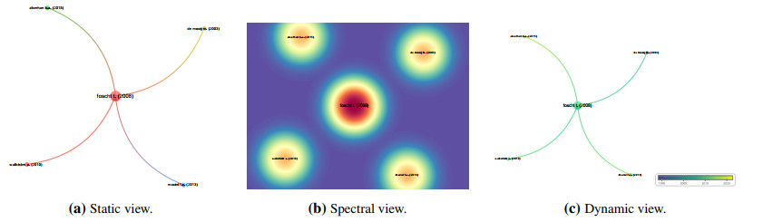
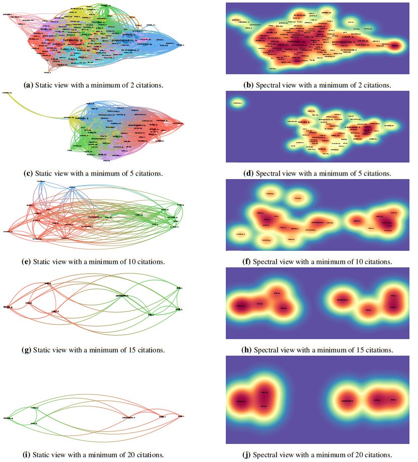
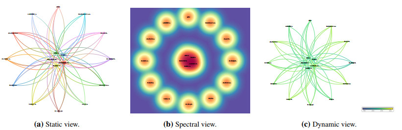
Combined with 12 additional authors identifiable in Figures 8a–8c, they constitute the group of most cited contributors. As affirmed by the overlay networks presented in Figures 6c–8c, offering a dynamic perspective of the citation analysis, the preponderance of nation brand and brand culture studies was amplified in the early 21st century. In turn, the co-citation analysis is performed by considering diversified values for the minimum number of times that a given published article is cited by academic peers (Figure 7). While the cloud of relevant authors is considerably large and dense when considering a minimum number of 2 citations (Figures 7a–7b), it becomes thinner and sparser as the threshold increases, forming two main clusters of authors at the supremum (i.e., when the minimum number is set at 20 citations). One cluster is composed of G. Hofstede, KL. Keller and JL. Aaker, while the other consists of N. Papadopoulos, S. Anholt and K. Dinnie. According to our empirical assessment, these six authors should be regarded as the most relevant contributors to the research field under scrutiny.
Figure 9 presents the network visualization map of the 65 most relevant terms observed in the title, abstract, and keywords of nation brand and brand culture studies. This map allows the identification of seven clusters in total, representing the diversity of themes in this research domain. Based on the cloud view presented in Figure 9a, each final group is labeled as follows:
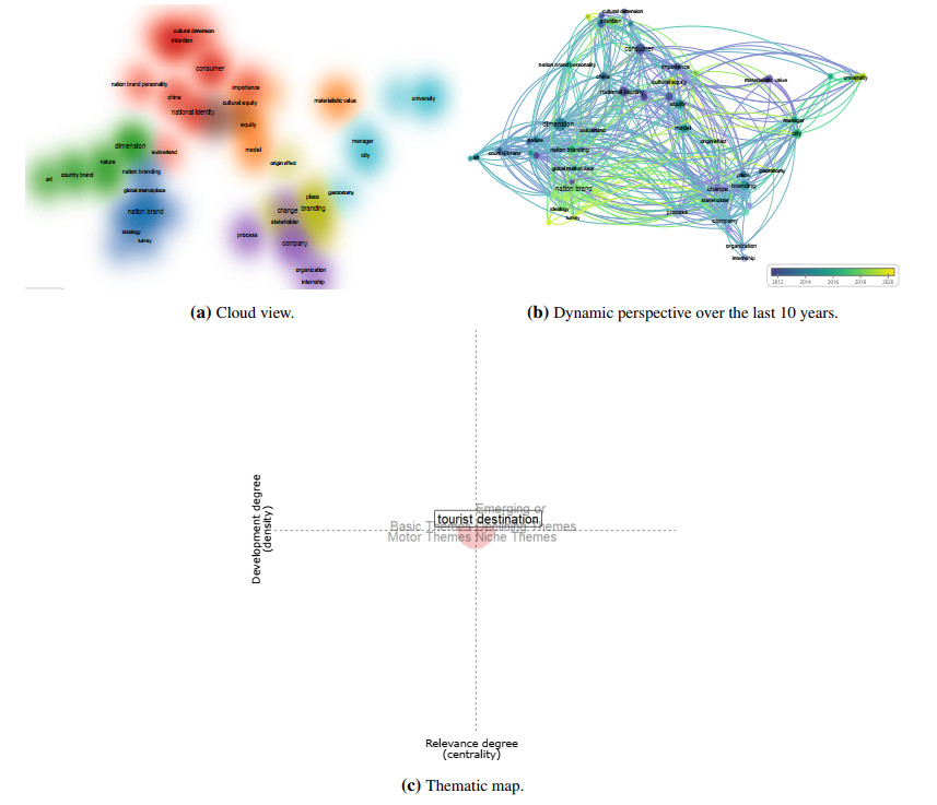
● Purple cluster - nation promoted as a country-of-origin brand: composed by representative terms of a firm-driven or production-based economy (e.g., company, business, vision, and organization);
● Yellow cluster - nation promoted as a city brand: composed by representative terms of regional marketing-based strategies (e.g., region, place branding, inter-regional brand, and origin effect);
● Red cluster - nation promoted as a consumption brand: composed by representative terms of consumption (e.g., consumer, behavioral intention, Japan, and experience);
● Orange cluster - nation promoted as a materialistic brand: composed by representative terms of materialism (e.g., materialistic value, consumer behavior, cultural equity, and Indian consumer);
● Green cluster - nation promoted as an environmental brand: composed by representative terms of sustainability and environmental action (e.g., nature, practitioner, technology, and nation brand molecule);
● Light blue cluster - nation promoted as a scientific brand: composed by representative terms of university as a key element of societal integration (e.g., university, public university, gastronomy, and students' identification); and
● Dark blue cluster - nation promoted as an ideological brand: composed by representative terms of ideological branding (e.g., ideology, transformation, power, hierarchy, and workforce diversity).
In turn, Figure 9b clarifies the evolution of each final cluster in the last decade. This graphical illustration reveals the:
● Historical seat occupied by purple, yellow, red, and orange clusters in the nation brand and brand culture field;
● Recent rise of green and blue clusters in the nation brand and brand culture field; in particular, the green cluster assumes a relevant role nearby 2015, while scientific and ideological clusters become important thematic groups especially after 2020.
Using the R-package provided by Aria and Cuccurullo (2017), Figure 9c presents the thematic map. Since co-word analysis draws clusters of keywords, they are considered as themes, whose density and centrality can be used in classifying themes and mapping them into a two-dimensional diagram. According to Cobo et al. (2011), Aria et al. (2020), and Aria et al. (2022), thematic maps are very intuitive plots that allow the analysis of themes according to the quadrant where they are placed: motor-themes belong to the upper-right quadrant, basic themes belong to the lower-right quadrant, emerging or disappearing themes belong to the lower-left quadrant, and very specialized (i.e., niche) themes belong to the upper-left quadrant. Interestingly, results suggest that the literature under scrutiny is characterized by the absence of themes belonging to any of these specific categories. This is because there is only one selected theme, tourist destination, that exhibits a neutral position in the thematic map, both with respect to density and centrality measures. It is thus evident that studies focusing on tourist destination are positioned around the central discourse of this literature and do not exhibit widespread dispersion. Intuitively, this result is justified by the fact that all studies in general tend to agree on the need of cities to attract tourists as a means of satisfying community-based needs. Therefore, marketing elements such as communication strategies, authenticity, and transparency are critical for successful country branding, yet these must be aligned with the unique cultural heritage and values of each nation. Main debated topics include social media and digital branding ecosystems within and across borders, experimentation of nation brand's conceptual image, the application of global, local, glocal and/or hybridized branding strategies in the destination place, branding research in emerging countries and bottom-of-the-pyramid markets, and the ability to reach local pockets of demand in emerging market. At a symbolic level, studies usually underscore that nation brands and brand culture can influence perceptions, attract investment, and facilitate cultural exchange, but it also internalizes concerns about oversimplification, appropriation, and commodification.
As depicted in Figure 9c, this theme tends to predominantly occupy a central location in the thematic map, indicating its interpretation as representative of all themes. This conclusion is consistent with the co-occurrence map analysis, where the theme is transversal across all clusters within the literature focused on nation brands and brand culture.
Measures of intra- and inter-cluster diversity are employed to assess statistically significant differences within and between clusters.
Intra-cluster measures. Table 1 presents descriptive statistics and intra-cluster outcomes associated with the knowledge base (i.e., total link strength of terms) of each cluster. It is evident that all diversity values fall below the threshold of 3.5, implying that all groups are characterized by a high degree of informational condensation. This outcome suggests that these clusters rely on very low diverse sources of information to formulate theories and interpretations, indicating that their underlying knowledge base is homogeneous. However, when compared to other alternatives, the higher value of diversity observed in representative clusters of ideological and consumption brands can be justified by the multidisciplinary nature implicit in both groups. On the other hand, the lowest value of diversity is observed in the materialistic brand cluster, indicating that studies promoting materialistic values tend to be quite homogeneous in their type of argumentation. In terms of evenness, each cluster sustains a value close to 1. These results indicate a moderately high apportionment between different categories, reflecting that each cluster is characterized by equally abundant terms. Intuitively, this suggests that each cluster enjoys an equitable degree of importance within the field under scrutiny. Regarding richness, the consumption brand cluster contains a higher number of terms (16) compared to the remaining alternatives. This result holds true due to the greater variety of case studies and countries captured by this cluster (e.g., China, Japan, and Switzerland).
| Cluster Type | |||||||
| Summary statistics (total link strengh) | Orange | Purple | Yellow | Dark Blue | Light Blue | Green | Red |
| Mean | 120.6667 | 137.5 | 120.75 | 134.5 | 149.4286 | 171.1 | 149.5 |
| Std. Dev. | 38.3597 | 79.7102 | 64.8289 | 50.3284 | 56.7094 | 105.9397 | 88.0682 |
| Min. | 62 | 20 | 40 | 64 | 43 | 40 | 20 |
| Max. | 164 | 269 | 233 | 230 | 230 | 448 | 286 |
| Skewness | -0.2611 | 0.0833 | 0.4621 | 0.5460 | -0.6475 | 1.8279 | 0.2911 |
| Kurtosis | 1.9842 | 2.2609 | 2.1889 | 2.4399 | 3.2227 | 6.0794 | 1.7576 |
| IQR | 58 | 102.5 | 92 | 64 | 46 | 30 | 148 |
| Intra-cluster metrics | Orange | Purple | Yellow | Dark Blue | Light Blue | Green | Red |
| Shannon Diversity (H') | 1.7471 | 1.9129 | 1.9523 | 2.2408 | 1.8730 | 2.1558 | 2.6005 |
| Evenness (E) | 0.9751 | 0.9199 | 0.9389 | 0.9732 | 0.9625 | 0.9362 | 0.9379 |
| Richness (S) | 6 | 8 | 8 | 10 | 7 | 10 | 16 |
| Inter-cluster outcomes | Orange | Purple | Yellow | Dark Blue | Light Blue | Green | Red |
| Orange ('materialistic-based') cluster | 1 | ||||||
| Purple ('firm-driven') cluster | 1.9613∗∗∗(9.0981)[1807] | 1 | |||||
| Yellow ('regional marketing-based') cluster | 1.9614∗∗∗(10.9347)[1625] | 1.9611∗(1.8539)[2041] | 1 | ||||
| Dark Blue ('ideology-based') cluster | 1.9613∗∗∗(34.2942)[1734] | 1.9612∗∗∗(18.7034)[1942] | 1.9614∗∗∗(15.9394)[1677] | 1 | |||
| Light Blue ('university-driven') cluster | 1.9614∗∗∗(8.4344)[1683] | 1.9612∗∗(2.2210)[1954] | 1.9613∗∗∗(2837)[1713] | 1.9610∗∗∗(26.1370)[2294] | 1 | ||
| Green ('sustainability-driven') cluster | 1.9610∗∗∗(24.0138)[2317] | 1.9609∗∗∗(12.3030)[2528] | 1.9610∗∗∗(10.0489)[2228] | 1.9608∗∗∗(5.2233)[2947] | 1.9608∗∗∗(16.8875)[2757] | 1 | |
| Red ('consumption-driven') cluster | 1.9610∗∗∗(56.2142)[2208] | 1.9610∗∗∗(37.8203)[2280] | 1.9612∗∗∗(34.6116)[1945] | 1.9606∗∗∗(25.0826)[3627] | 1.9608∗∗∗(48.9103)[2989] | 1.9606∗∗∗(26.2031)[3594] | 1 |
| Notes: *** p<0.01 ** p<0.05 * p<0.1. In relation to inter-cluster diversity outcomes, coefficient estimates are presented without parenthesis or brackets, t-statistics are displayed in parentheses and degrees of freedom are observed in brackets. IQR denotes interquartile range. | |||||||
 DownLoad:
CSV
DownLoad:
CSV
Inter-cluster comparison. Statistically significant differences between clusters are analyzed by applying the nonparametric t-test proposed by Hutcheson (1970). While inter-cluster diversity results are presented in Table 1, comparisons between clusters on a 2×2 basis are graphically illustrated in Figure 10. Assuming a significance level of 5%, results indicate statistically significant differences in diversity among all clusters, except for the relationship between the purple and yellow groups. The absence of a conceptual distinction between both clusters can be justified by the historical connection, actions, and communication channels shared between country-of-origin and city branding strategies. Additionally, this result empirically validates that differentiated nation brand strategies are not necessarily mutually exclusive.***
***Özsomer et al. (2012) confirm the similarity between actions of the private sector and the role of each local region in fostering a nation brand with the expectation to ensure global impact and international projection.
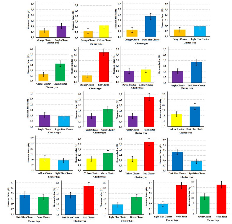
Since the null hypothesis of two homogeneous knowledge bases (i.e., the absence of inter-cluster diversity) is not rejected at a significance level of 5%, there is a notable sign of inter-cluster homogeneity for this specific case study.
Regarding RQ2, it can be concluded that the literature has predominantly emphasized six possible marketing strategies for a country to become a world-renowned brand:
1. Joint integration of country-of-origin and city branding;
2. Consumption branding;
3. Materialism branding;
4. Environmental branding;
5. University branding; and
6. Ideological branding.
Concerning RQ3, results indicate that the new green paradigm plays a leading role after the agreement signed by 193 countries on the 17 UN-SDGs in September 2015, but both university and ideology take the branding lead after 2020. Hence, this study confirms a recent trend characterized by the emergence of nation brand and brand culture relying on the enhancement and revitalization of higher education and national identity systems. Finally, low values of diversity suggest that the creation of a nation brand with global impact should accommodate more heterogeneous experiences. In terms of strategic guidelines, this result emphasizes the importance of becoming a Stackelberg leader in the branding race to generate added value for any national economy.
Prediction and classification of future research trends. Figure 11 illustrates some preliminary tasks and provides a graphical representation of LDA outputs for recent years.
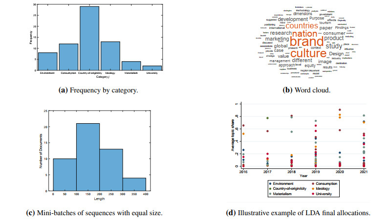
LDA assumes a prior β equal to 0.1, 1000 iterations with 10 samples, 50 iterations between samples, 3 seeds, 5 is set as the minimal word length and D=60 is the total number of articles. Also, recall that LDA infers the probability (i.e., relative strength) through which a given topic affects the allocation of each article to the set of possible clusters relying on text data information. Given the six final clusters identified in the Inter-cluster comparison subsection, it is assumed that 6 topics influence the allocation of each article to the set of clusters. Each topic is labeled as follows:
● Topic 1 reflects environmental concerns;
● Topic 2 materializes consumption concerns;
● Topic 3 captures the influence of country-of-origin and city-based concerns;
● Topic 4 reflects ideological concerns;
● Topic 5 captures materialism effects;
● Topic 6 materializes the relevance of universities,
and their combination defines the set of explanatory variables X used in the DCA. Before its execution, individual and joint significant tests exposed in Table 2 confirm that only Topic 1 (i.e., representative probabilities of environmental concerns) and Topic 2 (i.e., representative probabilities of consumption concerns) have explanatory power on the target variable's behavior. Table 2 also reveals failure to reject the null hypothesis in all Suest-based Hausman-McFadden tests, which implies that the dependent variable is legitimately composed of 6 categories. Estimated coefficients and marginal effects at the mean with the optimal − probit − model are shown in Table 2. In what follows, assume that the consumption cluster is the base category. For a significance level of 10%, the qualitative interpretation of estimated coefficients substantiates that, in comparison to the consumption cluster, a higher relative importance of:
| Consumption | Country-of-origin/city | Environment | Ideology | Materialism | University | |
| I. Statistical tests | ||||||
| Frequency | 1/5 | 5/12 | 7/60 | 11/60 | 1/20 | 1/30 |
| Suest-based Hausman | ϰ2[12]=4.494p=0.973 | ϰ2[12]=3.645p=0.989 | ϰ2[12]=4.980p=0.959 | ϰ2[12]=2.499p=0.998 | ϰ2[12]=1.705p=1.000 | ϰ2[12]=2.290p=0.999 |
| Individual significanceΨ | ϰ2[5]=14.830∗∗p=0.011 | ϰ2[5]=4.360p=0.499 | ϰ2[5]=12.160∗∗p=0.033 | ϰ2[5]=7.240p=0.203 | ϰ2[5]=5.850p=0.321 | ϰ2[5]=3.810p=0.577 |
| II. Coefficients | ||||||
| Consumption cluster normalized to zero | ||||||
| Intercept | 1.116∗∗(0.491) | −1.230(0.837) | 1.167(0.532) | 0.251(0.647) | −1.643(1.115) | |
| Topic 1 | −1.805∗∗(0.872) | −1.229(1.651) | −4.421∗∗∗(1.625) | −3.559∗(2.036) | −1.698(2.690) | |
| Topic 2 | 1.130(2.545) | 6.474∗∗(2.853) | −2.618∗∗(3.545) | −3.117(5.821) | 5.536∗(3.141) | |
| III. Marginal effects at the mean | ||||||
| Topic 1 | 0.508∗∗(0.203) | 0.017(0.270) | 0.080(0.179) | −0.506∗∗(0.223) | −0.106(0.122) | 0.007(0.111) |
| Topic 2 | −0.220(0.516) | 0.210(0.535) | 0.721∗∗(0.324) | −0.672∗(0.403) | −0.245(0.207) | 0.206(0.197) |
| IV. Qualitative metrics | ||||||
| Log Likelihood | −69.217 | |||||
| Notes: *** p<0.01 ** p<0.05 * p<0.1. Non-robust standard errors in parentheses since the method of estimation is maximum likelihood. The symbol Ψ serves to indicate that the joint significance test result for all regressors is ϰ2[30]=39.110 with p=0.123, the joint significance test result for all regressors except for Topics 1 and 2 is ϰ2[20]=19.180 with p=0.510 and the joint significance test result only for Topics 1 and 2 is ϰ2[10]=21.390 with p=0.019, thereby justifying the final deterministic component of the regression model β1+β2Topic1i+β3Topic2i for a critical p-value of 5%, with i={Article 1,...,Article 60}. | ||||||
DownLoad:
CSV
● The environmental topic is associated with a lower likelihood of city, ideological, and materialism branding, ceteris paribus;
● The consumption topic is associated with a lower likelihood of ideological and materialism branding and a higher likelihood of environmental branding, ceteris paribus.
Marginal effects at the mean displayed in Table 2 confirm similar findings, but from a quantitative point of view. Considering a critical p-value of 10% it is estimated that, for the article that exhibits average characteristics and holding everything else constant, the increase of one percentage point (p.p.) in the probability of coverage of content related to:
● Environmental concerns increases (decreases) the probability of belonging to the consumption (ideology) cluster by 50.8 (50.6) p.p., respectively;
● Consumption concerns increases (decreases) the probability of belonging to the environment (ideology) cluster by 72.1 (67.2) p.p., respectively.
A graphical illustration of the impact of both regressors on the mean preponderance of category j is presented in Figure 12. When the explanatory variable is the environment's relative importance, it is concluded that:
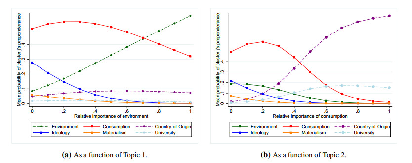
● For the case of minimal relative importance, it is estimated that consumption is the most prevalent cluster (∼ 55%), followed by ideology (∼ 30%), keeping all other categories with a relevance of less than 10%, ceteris paribus;
● When the relative importance reaches the maximum point, it is estimated that environment is the most prevalent cluster (∼ 60%), followed by consumption (∼ 30%), keeping all other categories with a relevance of less than 10%, ceteris paribus;
● As expected, there is a positive relationship between the representative cluster of environmental concerns and the relative importance of the environmental issue.
Focusing on the two clusters with the greatest preponderance, it is interesting to note that:
● There is a negative relationship between the representative cluster of ideology and the relative importance of the environmental issue;
● There is a non-monotonic (i.e., inverted-U) relation between the representative cluster of consumption and the relative importance of environmental issues. This result suggests that, in order to justify the need for greater environmental sustainability, the scientific discourse tends to dissuade brand consumption.
These findings reflect a trade-off between the environment and consumption/ideology: as the environmental concern becomes the core theme of a study, this will tend to lessen the importance of consumption and ideology in brand formation. When the consumption's relative importance is used to explain the target variable, evidence is found that:
● For the case of minimal relative importance, it is estimated that consumption is the most prevalent cluster (∼ 50%), ceteris paribus. This conclusion is not paradoxical given that, as confirmed by the results displayed in Content, this cluster has a strong historical root in the literature focused on country branding and brand culture so that, even when the content of a given article is unrelated to consumption brand, it can be classified as belonging to the consumption cluster;
● When the relative importance is minimal, it is estimated that approximately 20% of the scientific production is associated with ideological and environmental branding, while remaining all other categories with a relevance below 10%, ceteris paribus;
● When the relative importance reaches the maximum point, it is estimated that, country-of-origin/city is the most prevalent cluster (∼ 85%), followed by university (∼15%), keeping all other categories with a negligible relevance, ceteris paribus;
Moreover, there is a negative relation between the consumption's relative importance and ideological and environmental branding. It is also evident a positive relationship between the consumption's relative importance and university branding, which reflects that academic studies tend to overemphasize the andragogic role of higher education institutions (HEIs) in consumption branding contexts. Finally, there is a positive relationship between the consumption's relative importance and country-of-origin/city branding such that when the scientific discourse pretends to disseminate consumption idiosyncrasies, the importance of FDI decisions and place branding tends to be exacerbated.
Additional quantitative information, including average total citations per year, most productive countries and authors, annual scientific production, documents' co-citation analysis, journals' co-citation network, and networks of collaboration between authors, HEIs, and countries, is provided in Table A3 and Figures A1–A2 of the Appendix for interested readers.
Citation, inter-cluster, LDA, and DCA analyses empirically confirm that:
● The new green paradigm is gaining relevance in the field of nation brand and brand culture, particularly after 2015;
● Similar reasoning is applied to ideological branding, but only after 2020;
● Country-of-origin and city branding are not mutually exclusive strategies;
● There is trade-off between the relative importance of environmental content and the notoriety of ideological and consumption branding strategies.
Therefore, it is of paramount importance to articulate the quantitative assessment with a qualitative narrative underscoring the pivotal role played by nation brands and brand culture, typically situated within the realm of international marketing. These elements serve as catalysts, instigating innovation and transformation in green branding, and consequently, in harnessing the influential role of green finance. Specifically, these institutional elements allows us to identify two valuable niche opportunities for future research in the field of green finance: green nation brands and green brand culture. Moreover, both research opportunities are contextualized within a qualitative framework devised to accommodate ideological branding and its corresponding characteristics.
Conceptualization of green finance nation brand. The notion of green finance nation brand embodies a strategic vision for economic development that prioritizes environmental sustainability, fosters innovation, and contributes to global efforts in addressing climate change and other challenges faced by world nations, while having financial markets as supporting backbone (Failler and Li, 2019). It involves the integration of environmentally sustainable principles and practices within a nation's financial system, policies, and overall economic identity (Kemfert and Schmalz, 2019). This concept underscores the idea that a country can build and promote its global image by aligning its financial strategies with ecological sustainability at multiple hierarchical levels of the territory, including municipalities (Gorelick and Walmsley, 2020). A deeper reflection on this research opportunity leads to defining several strategic pillars. Embracing green finance as part of a nation's brand communicates a commitment to environmental responsibility. As suggested in Carlsen (2023), it signifies that the country recognizes the importance of sustainability not only for its citizens but also for the global community. By positioning itself as a green finance nation, a country can attract environmentally conscious investors and businesses. Green finance initiatives, such as sustainable bonds or investment funds, can appeal to those seeking ethical and sustainable opportunities (Desalegn, 2023). Indeed, green finance promotes investments in long-term sustainability, contributing to the nation's economic resilience. By diversifying the economy with sustainable practices, a country can be better prepared to face future challenges related to climate change and resource depletion. A nation that successfully integrates green finance into its national brand can position itself as a global leader in sustainable development. This leadership role can extend to influencing international agreements, setting standards, and collaborating with other nations to address global environmental issues. Integrating green finance into the national brand is an acknowledgment of climate change risks. By adopting sustainable financial practices, a nation can contribute to the mitigation of climate risks and demonstrate a proactive stance in addressing environmental challenges. A nation that actively engages in green finance builds trust and credibility on the global sphere. This can enhance its reputation as a responsible actor in international affairs and strengthen diplomatic ties, as environmental issues increasingly become central to supranational cooperation. The pursuit of green finance encourages innovation in renewable energy, sustainable infrastructure, and other environmentally friendly technologies. This can position a nation as a hub for green innovation, fostering stronger international partnerships, economic growth and competitiveness (Shugurov, 2023). A green finance nation brand can also emphasize social and economic inclusivity by promoting sustainable development that benefits all segments of society. This holistic vision should consider not only environmental aspect but also social and economic equity. Establishing a green finance nation brand requires the integration and coherence of policies across different sectors and economic activities, particularly in light of controversial topics such as low-carbon hydrogen (Moura and Soares, 2023). This can lead to a more unified approach in addressing environmental challenges and can serve as a benchmark model for other nations. As such, green finance nation brand is associated with asset allocations among green enterprises and environmental players in general to boost the symbolic image of a country's concern with the new green paradigm, notably in democratic societies (Bennink, 2023).
Proliferation of green brand culture. Green finance, as part of the nation's brand culture, emphasizes social responsibility and ethical financial practices. This connection extends to businesses and individuals, encouraging them to adopt environmentally conscious practices in their financial decisions, further reinforcing the green brand culture (Failler and Li, 2019). In turn, a green brand culture encourages sustainable lifestyles, and the integration of green finance complements this by providing financial mechanisms that support eco-friendly choices (Bellostas et al., 2023). This can include incentives for green business loans, or financial products that reward environmentally responsible behavior, and investments in sustainable energy systems (Haas et al., 2021). If that is the case, then green finance becomes a reflection of a broader cultural shift towards environmental awareness and responsibility. The nation's brand culture, infused with green values, contributes to changing societal norms, encouraging individuals and enterprises to consider the environmental impact of their financial decisions (Wang et al., 2023). The connection with green brand culture allows for the implementation of education and awareness programs that promote financial literacy with an emphasis on sustainable practices. This ensures that the population and business organizations are well-informed and engaged in supporting green finance initiatives (Dzhengiz, 2020). Moreover, green brand culture often incorporates symbols, icons, and imagery that represent environmental sustainability. These elements can be seamlessly integrated into the branding of green finance initiatives, creating a consistent visual identity that reinforces the nation's commitment to a sustainable future. As suggested in Ilić et al. (2019), green brand culture promotes international collaboration on sustainable goals. By aligning green finance with this cultural ethos, a nation can actively engage in global efforts to address environmental challenges, contributing to its reputation as a responsible and environmentally conscious actor on the world stage (Ezuma and Matthew, 2022). The integration of green finance into the green brand culture also contributes to the development of a cohesive national identity. At the board of directors level, this sense of belonging is frequently characterized by a commitment to sustainability, ethical practices, and a recognition of the interconnectedness of economic, social, and environmental well-being (Huang et al., 2023). As such, a green brand culture is likely become status quo as soon as the growth and intermediate effect of fintech development on supporting green innovation, energy efficiency, and green supply chains is effectively established at the community level.
Green resilience, politicization of green branding, and green national identity. Although the integration of green finance into a nation's brand culture can yield numerous benefits, potential limits and welfare issues may arise. Shifting to a green economy presents challenges, especially for industries heavily reliant on non-renewable resources, potentially leading to job displacement, economic transition problems, and social unrest. Swift changes in financial practices, like the introduction of new green financial instruments, pose risks to financial stability, requiring careful management to avoid disruptions. Green finance can introduce market volatility and uncertainties, impacting investor confidence and economic stability. Equal access to sustainable financial products is crucial to prevent socioeconomic disparities, as an increased focus on green initiatives may lead to greenwashing, undermining the credibility of genuine efforts. The transition to a green economy may also require significant technological advancements and infrastructure development, which may not be properly absorbed to be considered as integrant part of the brand culture. Countries with limited resources or outdated infrastructure may face challenges in keeping pace with the demands of a green finance-driven economic model. In particular, developing nations may face challenges in adopting and integrating these technologies, potentially leading to disparities in the pace of transition. As more nations adopt green finance strategies, there may be increased competition for green investments and sustainable technologies. Balancing global cooperation with the need to secure national interests in a competitive landscape can be a complex diplomatic challenge. While embracing green finance is essential for long-term sustainability, nations must navigate the balance between environmental responsibility and maintaining global economic competitiveness. Striking this balance can be challenging, particularly in industries where competitors may not adhere to the same environmental standards. Additionally, the success of green finance initiatives often depends on global cooperation. Limited collaboration between nations in adopting and enforcing sustainability standards can hinder the effectiveness of individual nations' efforts. Additionally, the green transition may inadvertently exacerbate social inequalities if not implemented with equity in mind. For example, if the cost of transitioning to green practices disproportionately affects certain socio-economic groups, it could lead to social tensions. Developing and implementing effective regulations for green finance can be complex. Striking the right balance between incentivizing sustainability and avoiding unintended consequences requires careful consideration and ongoing adjustments to policies. The shift to sustainable practices may lead to increased demand for certain resources, such as rare metals for renewable energy technologies. This could create new environmental challenges, including resource depletion and ecological impacts. {Relying on emerging green technologies carries risks, such as unanticipated environmental consequences} or reliance on technologies that may become obsolete. Ensuring the safety and long-term viability of these technologies is crucial. Public acceptance of green finance initiatives is essential for their success. If the public perceives these initiatives as burdensome or if there is resistance to change, the effectiveness of green finance policies may be compromised. Navigating these challenges requires a careful and adaptive approach, with policies designed to address potential welfare problems while maximizing the positive impact of green finance initiatives on economic, social, and environmental well-being.
Given these difficulties, it is urgent the prevalence of a positive correlation between the penetration of green brand culture and the degree of green identity. Aligned with the perspective of green resilience, the ascent of green brand culture is also closely tied to the political rise of green parties, which brings environmental values into policymaking. In turn, the rise of green parties reflects a societal shift towards environmental consciousness and sustainability, ultimately facilitating the persistence of a green national identity.
Whether being imagined (Anderson, 1983) or real (Gellner, 1994), nations are social constructs that contain individuals bounded by a sense of identity (Gould and Skinner, 2007). According to Aaker (1996), brand identity is a distinctive collection of associations that the manager aims to build and sustain. These associations are derived from strengths and weaknesses that are ingrained in tangible and intangible features of a nation's identity system (Gaggiotti et al., 2008). After the concept of nation being developed in the 19th century, national identity entered the cutting-edge vocabulary and is now widely used indiscriminately to indicate a variety of things (Bulmer and Buchanan-Oliver, 2010). This phenomenon helps a person grasp the respective place, being described by the conviction that this common sharing binds together different individuals from a given country (Kirloskar-Steinbach, 2019). In any case, national identity is not simply the impression of a common culture since it also catches the sense of belonging to a certain place (Grimson, 2010).
The canonical conceptualization of national identity draws on theories emerging from psychology, sociology, self-concept, and collective identity. Specifically, accentuation is ascribed to the social identity theory (SIT) brought by Tajfel and Turner (1979). Accordingly, national identity is a form of collective identification serving the purpose of binding people together inside a given community, providing them a feeling of enrollment. In this sense, Connor (1978) asserts that national identity is not a fixed view based on tangible assets, but rather a self-perspective about the country. As per Bartikowski et al. (2021), SIT might take different structures like strict or political personality. However, pertinence is given to the construction of national identity, which is the degree to which individuals relate to a specific country and favor its novel qualities over those of elective options (Keillor and Hult, 1999). National identity, despite having adjoining social construct conceptions among scholars (Papadopoulos et al., 2018), is influenced by a common perception of collective identity (Hanson and O'Dwyer, 2019). National identity encompasses various constructs like topophilia (Tuan, 1990), racism (Ouellet, 2007), animosity and xenophobia (Klein and Ettensoe, 1999), patriotism, local identity, and ethnocentrism (Kosterman and Feshbach, 1989).†††
†††Patriotism is the degree of dedicated love, connection, unwaveringness that individuals feel comparable to the home country, and is associated with support for conservative political parties (Bartikowski et al., 2021). It decides a status to forfeit for the home country and acts as a safeguard instrument (Druckman, 1994). Local identity alludes to the sensation of belongingness to a local community and distinguishing proof with its lifestyle. It mirrors the faith and respect for local traditions, history and customs, as well as the interest in local events (Lantz and Loeb, 1998). Ethnocentrism is a belief held by customers about the appropriateness of purchasing foreign-made products (Shimp and Sharma, 1987). To ethnocentric shoppers, buying imported products is morally wrong since it harms the homegrown economy, causes employment misfortunes, and is a traitorous activity (Winit et al., 2014).
Future trend: the rise of green ideological branding. Ideological branding explores the relationship between individual and collective perceptions of national identity. Two main perspectives define the literature covering ideological branding. On the one hand, a strand of research defends that individual and collective perceptions of national identity are likely to be disconnected (Wodak et al., 1999). National identity is constructed by every person and by the overall group, so that heterogeneity is likely to be observed. Moreover, discernments about national identity are expected to change in the long run given that experiences are mutable. Stalnaker (2002) contends that national identity is a construct that can be considered unessential based on the ground that numerous buyers, at least in developed countries, have global visions that transcend national boundaries. On the other hand, a contemporaneous view recognizes that a national identity is arranged in light of the social contract, being thus pertinent for the pursuit of national strategic goals. Therefore, national identity gives individuals significance for their lives and it might be fundamental for keeping a basic degree of self-respect and security (Nielsen, 1999). Furthermore, national identity has the ability to be a productive force in the general public, providing positive social capital and spillover effects, such as the superior degree of unforced cooperation, quicker flow of information and a more compiling functioning of public service institutions (Aldridge et al., 2002). In this sense, national identity is viewed as a creditable form of identification, being worth of examination in the context of branding approaches (Bulmer and Buchanan-Oliver, 2010). The absence of agreement on a definition for ideological branding is also seen in the confrontation between two showcasing gurus: Anholt (2002) contends that this concept is a fundamental condition in a globalized world, while Aronczyk (2008) claims that it comprises a delicate patriotism process that can be masterfully used by governments to achieve alternative ends.
As green parties gain political influence, they advocate for policies that prioritize green initiatives, including the integration of environmental considerations into the financial sector. Green parties, when in power, can enact legislation and create a policy framework that supports the development of green finance. This includes incentivizing sustainable investments, imposing regulations that encourage environmental responsibility, and fostering a conducive environment for green financial instruments. As explained in Volcic and Andrejevic (2011), the basic commitment of ideological branding is that verifiable forms of national identification can become anachronistic threats to contemporary monetary interests. Furthermore, the market can dissolve archaic forms of cultural struggles by disaggregating the collective bargaining embedded in the social contract into self-interested individuals and reassembling them to branded communities. Nevertheless, it is not dogmatically certain that ideological branding and political nationalism are totally unrelated, nor that acts of violence decrease when the public sector plays the role of business operator (Turner, 1994b). The notion of commercial nationalism outlined by Turner (1994a), Seo (2008, 2021), and White (2009) alludes to the utilization of patriot requests by business entities to differentiate their products in the context of a competitive and progressively interdependent global marketplace, which is likely to be sharpened in the 4.0 Industry era. The public offer of nationalism, which has turned into a typical topic in libertarian outlets worldwide in countless nations, addresses a reflexive type of national identity building. As detailed in Volcic and Andrejevic (2011), commercial nationalism corresponds to the choice of consuming a particular version of the national identification and this development can be integrated into the concept of green finance nation brand and green brand culture.
From one viewpoint, business entities sell nationalism to obtain abnormal profits. Alternatively, the state can be marked itself as a brand, thereby imposing a twofold rationale behind commercial nationalism. Moreover, ideological branding cannot be detached from legislative issues since it opens scope for the promulgation of several patriot features. The literature focused on commercial nationalism not only recognizes the historical relationship between capitalism and nation state, but also emphasizes how economic transformations (e.g., globalization, the decline of public service, and state-supported broadcasting in the neoliberalism era) and new forms of competition fostered by mixed oligopolies readjust the connection between ideological and commercial branding (Volcic, 2009). The wish to consider national identity as the target group in contemporaneous marketing activities has to do with the emergence of a safer style of governance, where being populist is seen as a way to attract and retain voters. Surely, this manifestation of opportunism makes sense if nationalism branding is treated as a matter of revealing the national identity, which undeniably ought to comprise of a collective process. Therefore, a national identity brand and its associated story is not just a static idea, but rather a development path that should embrace expectations of the local population, stakeholders and civil society. From a social corporatism perspective, several techniques can be used to impose nationalist ideas and domestic propaganda into a crowd. In the limit, communication and marketing can modify the concept of citizenship, which may never again be interpreted as a simple connection among individual and nation state with respect to obligations and rights, but it can incorporate new components of moral responsibility (e.g., preordained referendums; imposition of partial military mobilization).
Bringing these ideas into the prospective field of green finance nation brand and green brand culture, green ideological branding is likely to be more self-sustainable as the crowd engagement increases, and the political rise of green parties may signify a public mandate for environmental policies. Citizens, increasingly concerned about climate change and ecological sustainability, support political movements that prioritize green initiatives, including green finance. Green finance becomes a strategic pillar of economic growth as governments recognize the potential for sustainable investments to drive innovation, create jobs, and foster long-term economic resilience. Green parties are likely to integrate green finance into broader economic planning, emphasizing its role in achieving both environmental and economic goals. Nations that strategically position green finance as part of their economic growth under the influence of green parties can emerge as international leaders in sustainability. This not only enhances their global reputation but also allows them to play a leading role in shaping international agreements and standards related to green finance. Green parties advocating for green finance contribute to investor confidence by signaling stability and a commitment to sustainable practices. This can attract a new wave of investors interested in environmentally responsible opportunities, further supporting economic growth. With green parties in power, there is likely to be a greater emphasis on research, innovation, and technological advancements in the green sector. This can position the country as a hub for green technology, attracting investments and fostering economic growth through the development and export of sustainable technologies. Nevertheless, green parties often strive to strike a balance between economic development and environmental conservation. The integration of green finance into economic policies reflects a commitment to achieving both objectives, demonstrating a holistic approach to sustainable development. Green finance, as a strategic pillar, aligns with the long-term planning advocated by green parties. This involves not only immediate economic gains but also the establishment of resilient economic structures that can withstand the challenges posed by climate change and environmental degradation. Among these elements, civil society and local communities probably stand out. The connection between green finance nation branding and green brand culture reinforces a nation's commitment to sustainability across multiple dimensions. It creates a unified narrative that encompasses financial practices, cultural values, and societal norms, contributing to a comprehensive and enduring image of a responsible and environmentally conscious nation. In this context, the integration of green finance into a nation's brand aligns with the broader green brand culture, emphasizing a holistic commitment to sustainability.
This narrative extends beyond the financial sector to encompass various aspects of society, including business practices, consumer behavior, socio-economic trends, cultural values, and ideological resilience. Disruptions have consistently shaped the history, with over a dozen occurring in the past century. The aftermath of the COVID-19 pandemic lingers, and the world finds itself at a critical juncture, potentially facing a significant downturn in the business cycle or a continuation of recent inflationary trends. In these moments, decisive actions can steer a nation towards disproportionate degrowth, emphasizing the need for adaptable skills, irrespective of the disruption's nature. Drawing parallels with regions marked by military training, the importance of experimentation during times of peace is undeniable, highlighting that thorough preparation increases the likelihood of success in battles, so that proactive contingency planning before disruptions occurs is paramount. This foresight equips countries to be agile and well-prepared for various scenarios, including the inertia on allowing the penetration of a green brand culture, dramatic shifts in demand and variety tastes, or supply shortages. Anticipating future disruptions, stress-testing systems, and fostering adaptability enhances the ability to support citizens and safeguard market position. This is because, in the near future, only a strong green finance nation brand will be able to foster consumer and investor confidence in the commitment to sustainability. When the principles of green finance are aligned with the broader cultural values, it reinforces the notion that sustainability is deeply embedded in the national identity and not just a superficial or temporary trend. In conclusion, strategies for "country" marketers to cultivate resilience and adaptability include building an intentional nation brand, using granular data, measuring with an investor mindset, adopting omnichannel marketing, and embedding crisis reaction into agile strategic and critical thinking. Implementing these steps fosters a culture of resilience within a national jurisdiction, enabling it to rebound from setbacks effectively. Despite the challenges, the potential for growth and renewal is always present, waiting to be harnessed.
Future agenda: involving citizens around a green finance national identity. At this point, it should be clear to the interested reader why the selection of scientific content for this bibliometric analysis stopped in the summer of 2021: the empirical exercise uncovers a rising pattern favoring the expansion of environmental concerns, ideological branding and nationalist movements, which has been factually confirmed by several events that took place in 2022 and 2023, such as the Ukrainian-Russian war and the Israelian-Hamas conflict. In light of our empirical results, the proliferation of country-specific green national identities is likely to be sharpened in the near future due to the persistence of a perfect storm, whose main ingredients contemplate:
● Erosion of the social contract or, equivalently, decline of the welfare state combined with the fall of the sense of belonging at the community level;
● The 2008-2009 financial crisis leveraged by the COVID-19 pandemic and the subsequent civilizational wars that the world presently has to deal with.
The increasing porosity of any national border for FDI flows gives to ideological branding a remarkable sense of urgency. When a national identity is threatened by the dispersed character of manufacturing, outsourcing and transnational conglomerates, ideology fosters a sense of national uniqueness on habits and perceptions. While state-oriented broadcasting networks can be challenged by commercial broadcasters and anonymous actions, they end up becoming authentic marketing consultants and even try to find ways to influence the median citizen, despite commercialization forms of nationalism may not be aligned with public primary needs. Nevertheless, ideological branding can still be a disputable process, particularly in the event of concerns with a country's international image. In the context of green finance nation brand and green brand culture, two fundamental questions arise:
1. How can a nation assert its commitment to environmental consciousness when a significant portion of its population resides on the brink of poverty, and its citizens are reluctant to contribute financially to the green transition?
2. Conversely, how can a country be regarded as a credible international partner when its official discourse deliberately rejects interest in supporting the green transition, despite its citizens being willing to contribute financially to such initiatives?
Creating a green ideological brand and assessing its return on investment requires monitoring the population, while its effectiveness depends on the credibility of the governmental speech. Under this circumstance, ideological branding can emerge at full speed, from impacting individuals to mobilizing civil society. Unsurprisingly, the recent rise of neoliberalism in some European Union Member States seems to be marked by the gospel of individualism and sensationalism, which can be sharpened through the lens of a "dirty" green speech. As Clayton and Pontusson (1998) warn, non-credible actions affecting the green transition may lead to a profound decrease of government assistance programs due to the transfer of social duties from the public domain to the private sphere in the future. Navigating these challenges requires a careful and adaptive approach, with policies designed to address potential welfare problems while maximizing the positive impact of green finance initiatives on economic, social, and environmental well-being.
Proposal of a normative framework. Drawing from the gathered insights, we suggest incorporating a normative framework to align with the theoretical viewpoint that green finance as a research field should encompass both country branding and brand culture. Examining the emergence of countries as nation brands is a fascinating topic that has gained the attention of academic literature over the past decade (Steenkamp, 2019). The concept of country branding refers to strategic efforts of a national jurisdiction to shape and promote its image, reputation, and identity on the global sphere. It involves using marketing principles and techniques to enhance a country's attractiveness to various stakeholders, including tourists, investors, businesses, and potential residents. Therefore, developing a comprehensive framework for country branding is extremely important, and it requires to internalize various factors that influence a country's perception through the definition of:
● Objectives and scope, which define the specific aspects of the nation brand to be explored (e.g., economic competitiveness, cultural appeal, and political stability);
● Conceptual model, which outlines the key components and relationships within a nation brand (e.g., economic indicators, cultural heritage, governance, human development, environmental sustainability, innovation, and international relations);
● Research methodology, which sets all the possible techniques to collect and analyze data (e.g., quantitative surveys, qualitative interviews, focus groups, and expert assessments). A combination of primary and secondary research may be needed to gather a comprehensive understanding of the nation brand;
● Key indicators and metrics, which allows to identify relevant parameters that can be used to measure the nation brand's value (e.g., gross domestic product growth, employment rates, tourism arrivals, FDI, and global rankings);
● Different experimental studies, namely stakeholder analysis (i.e., identify the key stakeholders who influence and shape the nation brand, which can include citizens, government officials, business leaders, international organizations, tourists, investors, and media outlets in order to understand their perceptions, expectations, and experiences on country branding), benchmark analysis (i.e., compare the nation brand against other countries under the form of key indicators, perceptions, and reputation to gain insights into the relative strengths and weaknesses of the nation brand), strategy evaluation (i.e., assess the effectiveness of a nation's brand strategy and communication efforts, evaluate the alignment between the intended brand image and the perceived image, while identifying gaps and opportunities for improvement), and longitudinal analysis (i.e., conduct panel data studies to track changes in the nation brand over time among different countries, so as to infer trends and emerging patterns, and evaluate the impact of specific treatments or policies on the nation brand's notoriety);
● Policy recommendations and continuous monitoring, which aim to provide insights for policymakers, government agencies, and other relevant stakeholders. These suggestions may enhance the nation brand's value, and can focus on multiple areas (e.g., marketing campaigns, infrastructure development, policy reforms, cultural promotion, and sustainability initiatives). It also allows to establish a system for continuously assessing the nation brand's value and the effectiveness of implemented strategies. This step should be flexible enough to allow for ongoing refinement and adaptation.
Using a co-occurrence analysis, a thematic knowledge structure was established to gauge the degree of semantic similarities between keywords. Through an inter-cluster comparative evaluation, six content clusters were identified, delineating the green paradigm crucial for a nation to evolve into a globally recognized brand with a focus on sustainability (Figures 9a–9b). Moreover, dynamic capabilities required for navigating the green transition underscore the imperative of harnessing the concepts of green nation branding and cultivating a green brand culture. These thematic indicators offer a holistic perspective on the management process necessary for countries to adapt to the green transition successfully. This adaptation can be facilitated by deploying green strategies with either community-based, global, or glocal orientations, thereby catalyzing both structural and conjectural shifts in the development of green values within models aimed at enhancing national brand reputation. Collectively, these elements enable us to formulate and recommend the normative framework depicted in Figure 13.
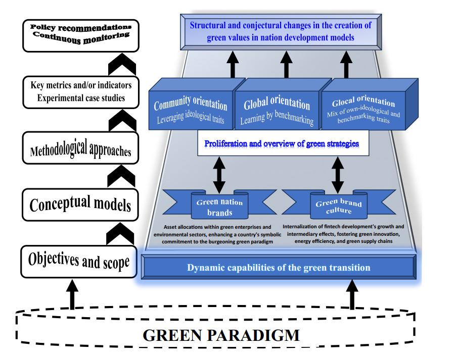
This study employs econometrics and computer science techniques to elucidate the evolution of studies focusing on nation brand and brand culture. The central research question aims to understand how a country succeeds in becoming a globally recognized brand. The recent emergence of green and ideological branding strategies delineates contemporary marketing tools for building the reputation of nation brands. Additional findings include the recognition that establishing a credible nation brand requires complementarity between horizontally differentiated clusters. Given these quantitative insights, a qualitative narrative delves on the rise of nation brands based on satisfying green finance principles, whose significance is likely to be heightened in the near future. Amid disruptions like the aftermath of COVID-19, proactive contingency planning becomes crucial for marketing organizations. The cultivation of a robust green brand culture enhances consumer and investor confidence by aligning principles of green finance with cultural values. Strategies for nations encompass intentional nation branding, data use, an investor mindset, omnichannel marketing, and incorporating crisis response into strategic thinking by internalizing green finance principles. Future research should explore citizens' involvement in shaping a green national identity, considering the rising trend of green ideological branding and nationalist movements. The convergence of challenges such as eroding social contracts, financial crises, and global conflicts may intensify the focus on ideological branding, especially in the context of environmental consciousness. Navigating these challenges demands careful, adaptive policies that address welfare problems and maximize social surplus.
Current bibliometric approaches are restricted to categorizing studies and their textual data. However, this limitation is highly restrictive because understanding the relationship between different content clusters is more relevant than merely segmenting them. Consequently, the primary technical implication of this study is to provide a rigorous quantitative protocol for inferring how the pattern of strategic substitutability and strategic complementarity between horizontally differentiated content clusters evolves. Achieving this purpose requires combining LDA with DCA in multinomial and unordered form, a methodology that, to the best of our knowledge, has not been used in bibliometric works prior to this study.
This innovation can also be explained from a mathematical point of view by offering a formal definition of strategic substitutability and strategic complementarity within the context of horizontally differentiated content clusters identified through a bibliometric analysis. Suppose a researcher strategically engages in intellectual activity to reduce reliance on a single type of content and ensure diversification to expand the existing literature. Then, consider a static game with complete information characterized by the following timing structure:
1. In the first stage, a researcher has the option to engage in effort k>0 to develop a second type of content aimed at enhancing the strand of literature under scrutiny.
2. In the second stage, if the researcher takes such action, then a Cournot game is played where publication quantities {y1,y2}∈R+0 are simultaneously and non-cooperatively chosen, resulting in net surpluses U1(y1,y2,k) and U2(y1,y2), respectively.
Note that U1(y1,y2,k) represents the researcher's net surplus after engaging in the initial action of developing a second type of content, while U2(y1,y2) represents the researcher's net surplus without engaging in effort to create a second type of content. In this scenario, the researcher operates as a monopolist, employing either null or positive effort to enhance the strand of literature under scrutiny. Hence, the researcher must make a strategic effort decision while recognizing the presence of competition to maximize net surplus for a given quantity of publications. This is the rationale for formally considering duopolistic competition between researcher 1 (potentially equipped with two types of content) and researcher 2 (equipped only with the pre-existing type of content). Let reaction functions be given by
| ˆy1:=ˆy1(y2,k),ˆy2:=ˆy2(y1) |
and suppose that there is a unique Nash equilibrium [y∗1(k),y∗2(k)] in the second stage satisfying the local stability condition
| |∂ˆy1∂y2∂ˆy2∂y1|<1. | (1) |
Additionally, suppose that
| ∂U1(y1,y2,k)∂y2<0,∂U2(y1,y2)∂y1<0, | (2) |
which are fairly standard assumptions in a competitive setting. By differentiating the equilibrium condition y∗1=ˆy1[ˆy2(y∗1),k] with respect to k, it follows that
| dy∗1(k)dk=∂ˆy1∂k1−∂ˆy1∂y2∂ˆy2∂y1. |
Using the envelope theorem, or equivalently, the first order condition ∂U2/∂y2=0, yields
| dU2[y∗1(k),y∗2(k)]dk=∂U2[y∗1(k),y∗2(k)]∂y1∂y∗1(k)∂k=∂U2[y∗1(k),y∗2(k)]∂y1∂ˆy1∂k1−∂ˆy1∂y2∂ˆy2∂y1. |
From Equations (1)–(2), one needs to satisfy
| ∂ˆy1∂k>0, | (3) |
to discourage the persistence of a single type of content, implying a negative effect of k on U2(⋅). Equations (3) implies that k represents a productive effort for researcher 1. Specifically, if there exists some k>0 such that U2[y∗1(k),y∗2(k)]<0, then the continuation of a single type of content is discouraged. However, investing in k>0 may be costly for researcher 1. Therefore, it is necessary to examine the impact of a higher value of k on researcher 1's net surplus. Using the envelope theorem and knowing that y∗2= ˆy2[ˆy1(y∗2,k)], yields
| dy∗2(k)dk=∂ˆy1∂k∂ˆy2∂y11−∂ˆy1∂y2∂ˆy2∂y1, |
and thus
| dU1[y∗1(k),y∗2(k),k]dk=∂U1[y∗1(k),y∗2(k),k]∂k+∂U1[y∗1(k),y∗2(k),k]∂y2∂ˆy1∂k∂ˆy2∂y11−∂ˆy1∂y2∂ˆy2∂y1. | (4) |
The first term on the right-hand side of Equation (4) represents a direct effect, while the second term denotes a strategic effect contingent upon the best response function of researcher 2. Two potential forms of retaliation exist, giving rise to the following definition.
Definition 1. In a given literature strand, strategic interaction is conceptualized as follows:
(i) Strategic complementarity. Content types 1 and 2 are strategic complements iff
| ∂ˆy2∂y1>0. |
(ii) Strategic substitutability. Content types 1 and 2 are strategic substitutes iff
| ∂ˆy2∂y1<0. |
All else being equal, a researcher has the incentive to identify and participate in the development of content types that exhibit strategic complementarity. This is because, under scenario (i), the quantity of publications of content type 2 increases with a marginal increase in the quantity of publications of content type 1. This allows the researcher to achieve his or her ultimate goal, which is to diversify content to maximize the chance of continued publishing in the long run within the strand of literature under scrutiny.‡‡‡
‡‡‡Conversely, under scenario (ii), the quantity of publications of content type 2 decreases with a marginal increase in the quantity of publications of content type 1. According to Equation (3), if y2 is a strategic substitute for y1, the strategic effect is positive. In light of Equation (4), if the direct effect is either positive or not excessively negative, then researcher 1 will expand k without hesitation to prevent the persistence of a single content type sustaining the strand of literature under scrutiny. Researcher 2 accommodates such a decision as long as the respective net surplus remains positive. However, this implies a business stealing effect in favor of researcher 1, who theoretically produces both types of content but will cannibalize towards content type 1. This situation does not arise under scenario (i) and contradicts the ultimate goal of researcher 1, which is the diversification of content to maximize the chance of continued publishing in the long run within the strand of literature under scrutiny.
Based on this mathematical formalization, it should now be clear that Figures 12a–12b encompass all potential strategic interaction patterns discussed within the literature pertaining to country branding and brand culture. Specifically, Figure 12a confirms that a marginal increase in environmental content correlates with a decrease in the prevalence of ideological, materialistic, and university clusters, indicating strategic substitutability. Conversely, a marginal increase in environmental content corresponds to a rise in the preponderance of country-of-origin and green clusters, suggesting strategic complementarity. Finally, there exists a non-monotonic relationship between the relative importance of environmental topics and the consumption cluster: its prevalence increases (decreases) for low (high) values of environmental topics, respectively. In turn, Figure 12b confirms that a marginal increase in consumption-related content correlates with a decrease in the prevalence of ideological, materialistic, and environmental clusters, implying strategic substitutability. Conversely, a marginal increase in consumption content corresponds to a rise in the preponderance of the country-of-origin cluster, indicating strategic complementarity. Finally, there exists a non-monotonic relationship between the relative importance of consumption topics and both consumption and university clusters, as their mean prevalence increases (decreases) for low (high) values of consumption-related content, respectively.
Moreover, it is necessary to coordinate the study's findings with the identification of real-world cases showcasing a set of differentiated marketing strategies and representative campaigns of country branding and brand culture. In particular, the following can be highlighted:
1. The There's Nothing Like Australia campaign clarifies the country's unique landscapes, wildlife, and cultural experiences, aimed at attracting tourists and promoting trade and investment opportunities;
2. The Marca Brasil campaign aims to promote tourism, festive events, and commercial activities of the country abroad;
3. The Canada's Food Guide campaign promotes Canadian cuisine and culinary experiences, targeted at food enthusiasts and culinary tourists;
4. The Germany Simply Inspiring campaign enhances the promotion of travel itineraries, events, and tourist attractions spanning all 16 provinces of Germany;
5. The 100% Pure New Zealand campaign highlighs the country's natural beauty and outdoor adventure activities, targeted at adventure-seeking tourists;
6. The Can'T Skip Tomorrow - Visit Portugal campaign leverages many endogenous resources (e.g., amazing water and waves; the value of cultural heritage and historical monuments; the purity of nature elements such as lakes, mountains, and landscapes; and art and gastronomic routes) that characterize this country;
7. The K-culture campaign promotes South Korea's K-pop, K-drama, and K-beauty to enhance the country's cultural soft power and attracting tourists and investment;
8. The Passion Made Possible campaign emphasizes Singapore's innovation, diversity, and connectivity, targeted at attracting tourists, businesses, and investors.
Furthermore, given the recent predominance of the green cluster, it can be concluded that assessing the impact and effectiveness of nation brand efforts is another critical aspect for stakeholders, practitioners, and scholars. These employ various methodologies, such as surveys, interviews, and content analysis, to measure brand perceptions, economic outcomes, tourism flows, and policy influence. These evaluations provide insights into the success and areas of improvement for country branding initiatives. Overall, performance outcomes may include the following:
● Changes in consumer perceptions and attitudes towards the nation brand's reputation;
● Changes in consumer behavior, such as tourism arrivals and tourism spending;
● Impacts on the nation's economic indicators, such as gross domestic product, employment, and FDI;
● Changes in diplomatic relations, foreign public opinion, and international relations;
● Impacts on the nation's competitiveness and positioning in the global marketplace;
● Effects on cultural exchange, HEI opportunities, talent attraction, and brain retention.
In recent years, there has been a burgeoning interest in the exploration of nation brand and brand culture research, underscored by a multidisciplinary and complementary approach, aligning it with broader literature such as national brands. The significance of fostering a competence networking, through engagement with esteemed researchers and affiliations, becomes unequivocally evident in its recent developments. The study also discerns six prevailing knowledge domains within the realm of this literature, five of which distinguished by their cohesive intra-group dynamics and notable inter-group heterogeneity. Furthermore, among the set of potential explanatory variables, only two topics satisfy multicollinearity and both individual and joint significance, culminating in the empirical demonstration that changes in the incidence of environmental and consumption topics engender both strategic substitutability and strategic complementarity effects in the allocation of scientific outputs between different content clusters. With that being said, it is now imperative to demystify certain fallacies that may obfuscate the perception of past and present research endeavors focused on country branding and brand culture. Together, these define what we call production, isolation, technical, complementarity–versus–substitutability, and hysteresis (PITCH) myths.
This myth attributes nation brand failures to the failure of private businesses. However, in reality, these failures stem from a failure of government, particularly public entities responsible for regulating and leveraging nation brand efforts. Maximizing social welfare and the value of a nation brand requires a deregulated market, at least in the short run equilibrium. When a government claims that leveraging a nation brand's value allows for wealth transfer from the rich to the poor, it actually redistributes wealth and income from both the extremely wealthy and the very poor to the middle class. Consequently, there are distortions at both ends of the economic spectrum in favor of the middle class, which represents the main source of market failures in any national economy (Friedman and Friedman, 1980). Hence, governmental actions to leverage the value of a nation brand may be ill-advised in this regard.
This myth suggests that high-quality research conducted by a single author is more valuable than research conducted collaboratively. The present analysis shows evidence that publishing studies that significantly improve the field of country branding is a challenging task. Moreover, the market for innovative ideas is scarce, making it more effective to enhance the reach of country branding research by directly contacting reputable researchers, clearly and thoroughly explaining the intended idea, and collaboratively developing it by relying on competence values (Ductor, 2015). This approach is entirely feasible, as demonstrated by influential researchers in the field who are generally affiliated with highly prestigious international HEIs and are open to collaborating with researchers from diverse geographical locations, provided that the research meets high-quality standards.
This myth emerges around the belief that nation brand studies should be expanded based on demand-side needs. A key finding from this empirical analysis reveals that most studies rely on surveys targeting the demand side of the market. However, it is essential to recognize that not only consumers contribute to shaping the reputation of a nation brand. Instead, people as individual agents are responsible for collectively influencing the concept-image of a nation brand, which includes consumers, producers, prosumers, immigrants, resident nationals, workers, and entrepreneurs. Regardless of how the nation brand evolves, such as through individual or business taxation, individual agents are the players who bear economic costs (Klein, 1978). Therefore, it is crucial to complement demand-side studies with supply-side analyzes that use real data from accountability reports of business organizations.
This myth assumes that powerful nation brands only follow the principle of maximum differentiation: countries either gain strength at the expense of weaker nation brands or enjoy international reputation through a full coordination scheme with other countries that share common interests. This study confirms the co-existence of complementarity and substitutability effects among different content clusters that materialize distinct forms of leveraging nation brands. From a political point of view, this means that nation brands become stronger by being both productive and attractive, often operating under a co-opetition environment. Furthermore, there has never been a period in history that has witnessed such a rapid and widespread improvement in country branding as seen today. From an economic perspective, this argumentation suggests that powerful nation brands may accommodate the nested principle of minimum–maximum differentiation (Ribeiro et al., 2016).
Adapting the approach advanced by Everett and Whitton (1952) to the realm of country branding, hysteresis is a concept which states that historical rates of a nation brand's value are likely to influence its current and future rates. In this sense, a hysteresis myth refers to a misconception or false belief related to the concept of hysteresis and its impact on the value of a nation brand. Readers holding a rushed reflection on the subject may claim that once a nation brand has experienced a decline in value, it is doomed to continue declining in the future. Intuitively, this myth suggests that if a nation brand has faced negative perceptions or a decline in its reputation in the past, it will inevitably continue to suffer from the same issues and be unable to recover. However, this myth fails to consider the dynamic nature of nation brands and their ability to adapt, change, and recover over time. While negative events or perceptions can have a statistically significant effect on a nation brand's value in the short run, it is not necessarily indicative of a permanent decline. Nation brands have the potential to implement effective strategies, engage in country branding campaigns, and address factors that led to the decline, thereby improving their reputation and restoring their value. Therefore, it is important to recognize that the concept of hysteresis is not an absolute rule when it comes to country branding and brand culture. It is one factor among many others that can influence the trajectory of a nation brand's value, and it should not be considered as the sole determinant of its success or failure.
Despite the effort to provide valuable contributions, this study may have limitations in the qualitative protocol. Recognizing that bibliographic details are integral to systematic reviews, Donato and Donato (2019) emphasize the importance of implementing high-quality research strategies to prevent formal errors. Recommended measures include involving at least one experienced bibliometric specialist, using the Peer Review of Electronic Search Strategies (PRESS) tool to validate information search strategies (Wolfswinkel et al., 2013), ensuring research strategies align with research questions, and assessing whether they are unconventional or complex (Dwivedi et al., 2008). Additionally, they stress the importance of using clear search terms, avoiding both excessive specificity and broadness, and correctly employing Boolean operators (Mohan and Ahlemann, 2011). To address uncertainties, robustness checks should be conducted. These may involve assessing whether accuracy can be enhanced by using proximity operators (e.g., adjacent, near, and within) or phrase search instead of relying solely on 'AND.' Researchers should also consider whether the limit between proximity operators is appropriate and whether any qualifiers are missing. Indeed, Hicks (1999) suggest that limitations in the qualitative protocol underscore the need for frequent systematic reviews. To facilitate the writing process, qualitative assessments can use the Preferred Reporting Items for Systematic Reviews and Meta-Analyses (PRISMA) protocol, accessible at http://prisma-statement.org/documents/PRISMA-P-checklist.pdf. This element is indispensable for ensuring consistency, transparency, and integrity, as it can be published in the prospective register of systematic reviews (PROSPERO). It serves as a valuable database for searching ongoing reviews, documenting systematic reviews, and preventing duplication. While repeating existing reviews may be redundant, there are circumstances where justifying a new review is necessary, particularly when methodological flaws are identified. Furthermore, certain academic journals mandate the inclusion of the PRISMA protocol registration number for publishing systematic reviews (Donato and Donato, 2019). Compared to primary research, systematic reviews offer the advantage of requiring fewer resources while enabling researchers not regularly involved in meta-analyses to undertake such studies. Although this study has followed a rigorous qualitative protocol, the above argumentation, along with the limited literature reviews and bibliometric analyses on this subject as confirmed by the Table A1 in Appendix, indicate that there is still more ground to cover. By conducting additional reviews focused specifically on country branding and brand culture, researchers can contribute to the advancement of knowledge in this area. Such a conduct could potentially uncover new insights and provide a more comprehensive understanding of the topic. Lastly, a content analysis applied to the discourse of researchers and practitioners can help us to understand who holds more influence on promoting and improving this research domain. Similarly, deep learning models can be employed to validate future trends and alternative research avenues.
V. M. Ribeiro acknowledges financial support from the FCT project DSAIPA-CS-0086-2020. Any necessary material for replication of this study can be provided upon request to vsribeiro@fep.up.pt. V. M. Ribeiro also appreciates the comments and suggestions from two anonymous reviewers, the Editor-in-Chief, the Editor-in-Charge, the Assistant Editor, and the English Editor, which substantially improved the quality of the final version of this manuscript.
The author declares that he has not used artificial intelligence (AI) tools in the creation of this article.
The author declares that there are no conflicts of interest.
| Author | Article | Area of research | Year | Topic |
| Karrh (1998) | Brand placement: A review | Business, Management and Accounting | 1998 | Review of place branding and related variants |
| Dinnie et al. (2004a) | Place branding: Overview of an emerging literature | Business, Management and Accounting | 2004 | Review of place branding and related variants |
| Dinnie et al. (2004b) | Country-of-origin 1965-2004: A literature review | Business, Management and Accounting | 2004 | Review of the country-of-origin theme |
| Guzman (2005) | A brand building literature review | Social Sciences | 2005 | Generical review on brand building |
| Chabowski et al. (2013) | A bibliometric analysis of the global branding literature and a research agenda | Social Sciences | 2013 | Bibliometric analysis of global branding |
| Papadopoulos et al. (2016) | Nation branding for foreign direct investment:an Integrative review and directions for research and strategy | Business and Economics | 2016 | Review of nation brand literaturefocusing on FDI |
| White et al. (2016) | Trends in international strategic management research from 2000 to 2013:Text mining and bibliometric analyses | Business, Management and Accounting | 2016 | Review of strategic management researchwith a brief coverage of nation image |
| Hao et al. (2021) | Two decades of research on nation branding: A review and future research agenda | Business, Management and Accounting | 2021 | Review of country branding |
| He et al. (2021) | Building the connection between nation and commercial brand:an integrative review and future research directions | Business, Management and Accounting | 2021 | Proposal of a coordination frameworkbetween nation and commercial branding |
| Södergren (2021) | Brand authenticity: 25 Years of research | Business, Management and Accounting | 2021 | Review on brand autheticity |
| Rojas-Méndez and Khoshnevis (2023) | Conceptualizing nation branding: the systematic literature review | Business, Management and Accounting | 2023 | Systematic literature review on nation branding |
DownLoad:
CSV
| [Ranking] Authors (Year) | Title | Journal | Cited by |
| [1] Mooij (2003) | Convergence and divergence in consumer behaviour: Implications for global advertising | International Journal of Advertising | 88 |
| [2] Matzler et al. (2016) | Brand personality and culture: The role of cultural differences on the impact of brand personality perceptions on tourists' visit intentions | Tourism Management | 87 |
| [3] Anholt (2005) | Anholt nation brands index: How does the world see America? | Journal of Advertising Research | 58 |
| [4] Gupta (2011) | Globalization does lead to change in consumer behavior: An empirical evidence of impact of globalization on changing materialistic values in Indian consumers and its aftereffects | Asia Pacific Journal of Marketing and Logistics | 49 |
| [5] Foscht et al. (2008) | The impact of culture on brand perceptions: A six-nation study | Journal of Product&Brand Management | 49 |
| [6] Rojas-Méndez (2016) | The nation brand molecule | Journal of Product&Brand Management | 29 |
| [7] Geary (2013) | Incredible India in a global age: The cultural politics of image branding in tourism | Tourist Studies | 25 |
| [8] Hsieh and Lindridge (2005) | Universal appeals with local specifications | Journal of Product&Brand Management | 22 |
| [9] Clifton (2014) | Towards a holistic understanding of county of origin effects? Branding of the region, branding from the region | Journal of Destination Marketing and Management | 18 |
| [10] Wilson and Hollensen (2010) | Saipa Group, Iran - using strategic brand extensions to build relationships | Journal of Islamic Marketing | 18 |
| [11] Gong et al. (2014) | Global use and access of social networking web sites: A national culture perspective | Journal of Research in Interactive Marketing | 15 |
| [12] Bulmer and Buchanan-Oliver (2010) | Experiences of brands and national identity | Australasian Marketing Journal | 14 |
| [13] Therkelsen and Gram (2010) | Branding Europe - between nations, regions and continents | Scandinavian Journal of Hospitality and Tourism | 12 |
| [14] Pearson and Pearson (2017) | Branding Food Culture: UNESCO Creative Cities of Gastronomy | Journal of Food Products Marketing | 11 |
| [15] Perez et al. (2011) | Intergenerational influence on brand preferences | Journal of Product & Brand Management | 11 |
| [16] Kaufmann and Durst (2008) | Developing inter-regional brands | EuroMed Journal of Business | 11 |
| [17] Martínez (2016) | Towards a network place branding through multiple stakeholders and based on cultural identities: The case of "The Coffee Cultural Landscape" in Colombia | Journal of Place Management and Development | 10 |
| [18] Song and Sung (2013) | Antecedents of nation brand personality | Corporate Reputation Review | 10 |
| [19] Smith and West (1994) | The globalization of furniture industries/markets | Journal of Global Marketing | 10 |
DownLoad:
CSV
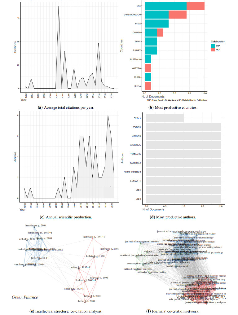
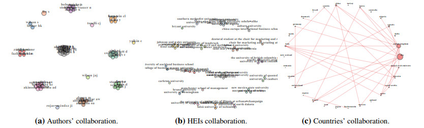
| Description | Results |
| Timespan | 1992 : 2021 |
| Sources (Journals, Books, etc) | 45 |
| Documents | 60 |
| Annual Growth Rate % | 2.42 |
| Document Average Age | 10.5 |
| Average citations per doc | 10.67 |
| Average citations per year per doc | 0.8208 |
| References | 2989 |
| Keywords Plus (ID) | 23 |
| Author's Keywords (DE) | 221 |
| Authors | 133 |
| Author Appearances | 142 |
| Authors of single-authored docs | 19 |
| Single-authored docs | 19 |
| Documents per Author | 0.451 |
| Co-Authors per Doc | 2.37 |
| International co-authorships % | 21.67 |
DownLoad:
CSV
Overall, additional quantitative results suggest that: the intellectual structure of studies is organized around two main groups, there are three main groups of co-cited academic journals, there are authors who prefer to work alone, but there are also collaboration networks that accommodate up to six members, there are HEIs who prefer to work alone, but there are also collaboration networks that accommodate up to five members, and the United States of America and the United Kingdom dominate the dissemination of content on nation brands and brand culture.
| [1] |
Silva AM, Silva MLN, Curi N, et al. (2005) Perdas de solo, água, nutrientes e carbono orgânico em Cambissolo e Latossolo sob chuva natural. Pesq Agrop Bra 40: 1223-1230. doi: 10.1590/S0100-204X2005001200010

|
| [2] |
Karydas C, Sekuloska T, Silleos G (2009) Quantification and site-specification of the support practice factor when mapping soil erosion risk associated with olive plantations in the Mediterranean island of Crete. Environ Monit Assess 149: 19-28. doi: 10.1007/s10661-008-0179-8
|
| [3] | Ganasri BP, Ramesh H (2015) Assessment of soil erosion by RUSLE model using remote sensing and GIS—A case study of Nethravathi Basin. Geosc Front: 1-9. |
| [4] |
Lin BS, Thomas K, Chen CK, et al. (2016) Evaluation of soil erosion risk for watershed management in Shenmu watershed, central Taiwan using USLE model parameters. Paddy Water Environ 14: 19-43. doi: 10.1007/s10333-014-0476-5
|
| [5] | Markose VJ, Jayappa KS (2016) Soil loss estimation and prioritization of sub-watersheds of Kali River basin, Karnataka, India, using RUSLE and GIS. Environ Monit Assess: 188-225. |
| [6] |
Rahman MR, Shi ZH, Chong C (2009) Soil erosion hazard evaluation: an integrated use of remote sensing, GIS and statistical approaches with biophysical parameters towards management strategies. Ecol Modell 220: 1724-1734. doi: 10.1016/j.ecolmodel.2009.04.004
|
| [7] |
Peter HBC, Chandler JH, Armstrong A (2010) Applying close range digital photogrammetry in soil erosion studies. Photogramm Rec 25: 240-265. doi: 10.1111/j.1477-9730.2010.00584.x
|
| [8] | Wischmeier WH, Smith DD (1965) Predicting Rainfall-Erosion Losses from Gopland East of the Rocky Mountains. Agri Hand 282: 47. |
| [9] | Strand RI, Pemberton EL (1982) Reservoir sedimentation: Technical guidelines for Bureau of Reclamation. U.S. Bureau of Reclamation, Denver. |
| [10] |
Ananda J, Herath G (2003) Soil erosion in developing countries: a socio-economic appraisal. J Environ Manag 68: 343-353. doi: 10.1016/S0301-4797(03)00082-3
|
| [11] | Humberto BC, Rattan L (2008) Water erosion. In: Principles of soil conservation and management. Springer, New York, 21-53. |
| [12] | Jinren RN, Yingkui KL (2003) Approach to soil erosion assessment in terms of land-use structure changes. J Soil Water Conserv 58: 158-169. |
| [13] |
Prasannakumar V, Shiny R, Geetha N, et al. (2011) Spatial prediction of soil erosion risk by remote sensing, GIS and RUSLE approach: A case study of Siruvani River watershed in Attapady valley, Kerala, India. Envir Ear Sc 64: 965-972. doi: 10.1007/s12665-011-0913-3
|
| [14] |
Chen T, Niu R, Ni P, et al. (2011) Regional soil erosion risk mapping using RUSLE, GIS, and remote sensing: A case study in Miyun Watershed, North China. Envir Ear Sc 63: 533-541. doi: 10.1007/s12665-010-0715-z
|
| [15] | Beskow S, Mello CR, Norton LD, et al. (2009) Soil erosion prediction in the Grande River Basin. Brazil using distributed modeling. Catena 79: 49-59. |
| [16] |
Cohen MJ, Shepherd KD, Walsh MG (2005) Empirical reformulation of the universal soil loss equation for erosion risk assessment in a tropical watershed. Geoderma 124: 235-252. doi: 10.1016/j.geoderma.2004.05.003
|
| [17] | Werneck Lima JEF, Lopes WTA, Aquino FG, et al. (2014) Assessing the use of erosion modeling to support payment for environmental services programs. J of Soils and Sed 14: 1258-1265. |
| [18] | Mellerowicz KT, Rees HW, Chow TL, et al. (1994) Soil conservation planning at the watershed level using the Universal Soil Loss Equation with GIS and microcomputer technologies: a case study. J Soil Water Conser 49: 194-200. |
| [19] | Ha NM (2011) Application of USLE and GIS tool to predict soil erosion potential and proposal land cover solutions to reduce soil loss in Tay Nguyen. FIG Conference—Bridging the Gap Between Cultures—Marrakech, Morocco. |
| [20] | Karydas CG, Sekuloska T, Sarakiotis I (2005) Fine scale mapping of agricultural landscape features to be used in environmental risk assessment in an olive cultivation area. IASME Trans 2: 582-589. |
| [21] |
Mati BM, Veihe A (2001) Application of the USLE in a savannah environment: comparative experiences from East and West Africa. Singap J Trop Geogr 22: 138-155. doi: 10.1111/1467-9493.00099
|
| [22] |
Angima SD, Stott DE, O'Neill MK, et al. (2003) Soil erosion prediction using RUSLE for central Kenyan highland conditions. Agric Ecosyst Environ 97: 295-308. doi: 10.1016/S0167-8809(03)00011-2
|
| [23] |
Kothyari UC, Tewari AK, Singh R (1994) Prediction of sediment yield. J of Irrig and Drain Eng ASCE 120: 1122-1131. doi: 10.1061/(ASCE)0733-9437(1994)120:6(1122)
|
| [24] | Pandolfo C, Braga HJ, Silva Junior VP, et al. (2002) Atlas climático digital do Estado de Santa Catarina. Florianópolis: Epagri. CD-Rom. |
| [25] | Pinheiro A, Kaufmann V, Perazzoli M, et al. (2010) Avaliação dos escoamentos em diferentes escalas espaciais na bacia do ribeirão Concórdia [Evaluation of flows in diferentes patialscales in the Concórdia creek basin]. In X Symposium of Water Resources of Nordeste, Fortaleza 1: 1-11. Porto Alegre Brazil: ABRH. |
| [26] | Klein RM, Rodriguez HB (1978) Mapa Fitogeográfico do Estado de Santa Catarina [Phytogeographic map of the state of Santa Catarina]. In Mapa Fitogeográfico do Estado de Santa Catarina. Imprensa Oficial do Estado de Santa Catarina. IOESC. Florianópolis, SC, Brazil. |
| [27] | Wischmeier WH, Smith DD (1978) Predicting rainfall erosion losses: a guide to conservation planning. Agric Handb 537, Washington-D.C: USDA. 57 p. |
| [28] |
Renard KG, Freimund JR (1994) Using monthly precipitation data to estimate the R-factor in the reviser USLE. J of Hydr 157: 287-306. doi: 10.1016/0022-1694(94)90110-4
|
| [29] |
Kim JB, Saunders P, Finn JT (2005) Rapid Assessment of soil erosion in the rio Lempa Basin, Central America, Using the Universal Soil Loss equation and Geographic Information Systems. Envir Manag 36: 872-885. doi: 10.1007/s00267-002-0065-z
|
| [30] | Bertoni J, Lombardi Neto F (1998) Conservação do solo. 4. ed. São Paulo: Ícone Ed., 392 p. |
| [31] | Denardin JE (1990) Erodibilidade de solo estimada por meio de parâmetros físicos e químicos. 81p. Thesis (Doctored em Agronomy—Soil and Nutrition of Plants)—Escola Superior de Agricultura Luiz de Queiroz, Univ. de São Paulo, Piracicaba. |
| [32] | Caputo HP (1988) Mecânica dos Solos e suas aplicações. Fundamentos. 6º edição, Rio de Janeiro: Livros Técnicos e Científicos Editora. |
| [33] | Galindo ICL, Margolis E (1989) Tolerância de perdas por erosão para solos do Estado de Pernambuco. Rev Bra de Ciê do Solo 13: 95-100. |
| [34] | Alexakis DD, Hadjimitsis DG, Agapiou A (2013) Integrated use of remote sensing, GIS and precipitation data for the assessment of soil erosion rate in the catchment area of “Yialias” in Cyprus. Atm Resea 131: 108-124. |
| [35] | Ranzi R, Hung Le T, Rulli MC (2012) A RUSLE approach to model suspended sediment load in the Lo River (Vietnam): effects of reservoirs and land use changes. J of Hydrol: 422-423. |
| [36] | Paiva EMC, Paiva JBD (2001) Hidrologia aplicada à gestão de pequenas bacias hidrográficas. Porto Alegre: ABRH, 367 p. |
| [37] | Williams JR, Berndt HD (1977) Determining the universal soil equation`s length-slop factor for watershed. In: Soil Erosion: prediction and control. Ankeny: Soil Conservation Society of America: 217-255. |
| [38] |
Bertol I, Shick J, Batistela O (2002) Razão de perdas de solo e Fator C para milho e aveia em rotação com outras culturas em três tipos de preparo de solo. Rev Bra de Ciê de Solo 26: 545-552. doi: 10.1590/S0100-06832002000200029
|
| [39] | Martins SG, Silva MLN, Avanzi JC, et al. (2010) Fator cobertura e manejo do solo e perdas de solo e água em cultivo de eucalipto e em Mata Atlântica nos Tabuleiros Costeiros do Estado do Espírito Santo. Scien. Forest 38: 517-526. |
| [40] | Stein DP, Donzelli PL, Gimenez AF, et al. (1987) Potencial de erosão laminar, natural e antrópico, na Bacia do Peixe-Paranapanema. Anais 4º Simpósio Nacional de Controle de Erosão. Marília-SP: ABGE/DAEE: 105-135. |
| [41] | Tomzani JC, Mantovani LE, Bittencourt AVL, et al. (2005) Sistematização dos fatores da Eups em SIG para quantificação da erosão laminar na bacia do rio Anta Gorda (PR). Est Geog 3: 1-21. |
| [42] | Morgan RPC (1995) Soil erosion and Conservation. Longman Group Limited, 2 ed. |
| [43] | Silva AM, Schulz HE, Camargo PB (2007) Erosão e hidrossedimentologia em bacias hidrográficas. 2. Ed. São Carlos-SP: RiMa, 158 p. |
| [44] |
Strand GH, Dramstad W, Engan G (2002) The effect of field experience on the accuracy of identifying land cover types in aerial photographs. Int J Appl Earth Obs Geoinf 4: 137-146. doi: 10.1016/S0303-2434(02)00011-9
|
| [45] | Wanielista MP (1978) Storm water management: quality and quantity, Ann Arbor Science, 383 p. |
| [46] | Ali SA, Hagos H (2016) Estimation of soil erosion using USLE and GIS in Awassa catchment, Rift valley, Central Ethiopia. Geod Reg 7: 159-166. |
| [47] |
Berberoglu S (2003) Sustainable management for the Eastern Mediterranean coast of Turkey. Env Manag 31: 442-451. doi: 10.1007/s00267-002-2724-5
|
| [48] | Ali SA, Tesgaya D (2010) Landuse and landcover change detection between 1985–2005 in parts of Highland of Eastern Ethiopia using remote sensing and GIS techniques. Int J Geoinf 6: 35-40. |
| [49] |
Meshesha DT, Tsunekawa A, Tsubo M, et al. (2014) Land use change and its socio-environmental impact in Eastern Ethiopia’s Highland. Reg Environ Chang 14: 757-768. doi: 10.1007/s10113-013-0535-2
|
| [50] |
Evrendilek F, Doygun H (2000) Assessing major ecosystem types and the challenge of sustainability in Turkey. Env Manag 26: 479-489. doi: 10.1007/s002670010106
|
| [51] | Wali MK, Safaya NM, Evrendilek F (2002) Ecological rehabilitation and restoration in the Americas with special reference to the United States of America. In: Perrow MR, Davy AJ (Eds.) Handbook of Rest Ec 2. Cambridge University Press, Cambridge, 3-31. |
| [52] | Yang CT (1996) Sediment Transport: Theory and Practice. McGraw-Hill Book Company, Inc, New York. |
| [53] | EMBRAPA (1997) Manual de métodos de análise de solo. Rio de Janeiro. 2. ed. rev. EMBRAPA: 212 p. |
| [54] | Yang CT (1973) Incipient motion and sediment transport. J of the Hyd Div 99: 1679-1701. |
| [55] | Silva CR, Bressiani DA, Bettiol GM S, et al. (2014) Aplicação do Modelo SWAT (Soil and Water Assessment Tool) para estimar produção de sedimento e nutrientes na Microbacia Experimental da EMBRAPA Pecuária Sudeste. Simpósio Nacional de Instrumentação Agropecuária. São Carlos: 609-612. |
| [56] | Silva CR (2010) Aplicação do Modelo SWAT para estimar produção de sedimentos e transporte de fósforo e nitrogênio na microbacia do Ribeirão Canchim—EMBRAPA Pecuária Sudeste. Dissertação (Mestrado)—Escola de Engenharia de São Carlos, Universidade de São Paulo, São Carlos. |
| [57] | Vieira VF (2008) Estimativa de perdas de solo por erosão hídrica em uma sub-bacia hidrográfica. Geografia 17: 73-81. |
| [58] | Oliveira VA, Mello CR, Durões MF, et al. (2014) Vulnerabilidade a erosão do solo na bacia do rio Verde, Minas Gerais do Sul. Ciê Agrotec 38. |
| [59] | Pradeep GS, Ninu Krishnan MV, Vijith H (2014) Identification of critical soil erosion prone areas and annual average soil loss in an upland agricultural watershed of Western Ghats, using analytical hierarchy process (AHP) and RUSLE techniques. Arab J of Geosc 8: 3697-3711. |
| [60] | Gilles L, Cogo NP, Bissani CA, et al. (2009) Perdas de água, solo, matéria orgânica e nutriente por erosão hídrica na cultura do milho implantada em área de campo nativo, influenciadas por métodos de preparo do solo e tipos de adubação. Rev Bra de Ciê do Solo 33, p. 1427-1440. |
| [61] | Adinarayana J (2003) Spatial decision support system for identifying priority sites for watershed management schemes. In First interagency conference on research in the watersheds (ICRW) Arizona: Benson: 405-408. |
| [62] |
Silva RM, Santos CAG, Montenegro SMGL (2012). Integration of GIS and remote sensing for estimation of soil loss and prioritization of critical sub-catchments: a case study of Tapacura catchment. Nat Haz 62: 953-970. doi: 10.1007/s11069-012-0128-2
|
| [63] |
Patel DP, Gajjar CA, Srivastava PK (2013) Prioritization of Malesari mini-watersheds through morphometric analysis: a remote sensing and GIS perspective. Env Ear Sc 69: 2643-2656. doi: 10.1007/s12665-012-2086-0
|
| [64] |
Khadse GK, Vijay R, Labhasetwar PK (2015) Prioritization of catchments based on soil erosion using remote sensing and GIS. Env Monit and Assess 187: 333. doi: 10.1007/s10661-015-4545-z
|
| 1. | Nini Johana Marín-Rodríguez, Juan David González-Ruiz, Sergio Botero, Evolution of Green Finance: Mapping Its Role as a Catalyst for Economic Growth and Innovation, 2024, 17, 1911-8074, 507, 10.3390/jrfm17110507 | |
| 2. | Hsu-Hsin Chiang, Chung-Hui Tseng, The Approach to Enhance Brand Citizenship Behavior and Customer-Based Brand Equity: Multilevel Mediating Effects in International Tourist Hotels, 2025, 1525-6480, 1, 10.1080/15256480.2025.2513869 |
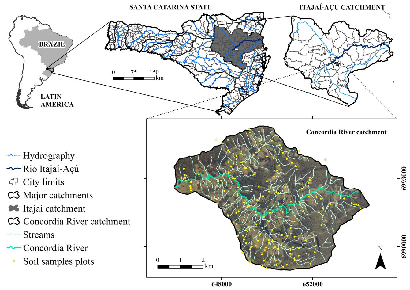
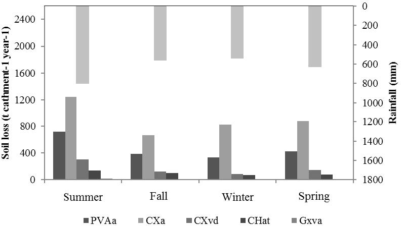
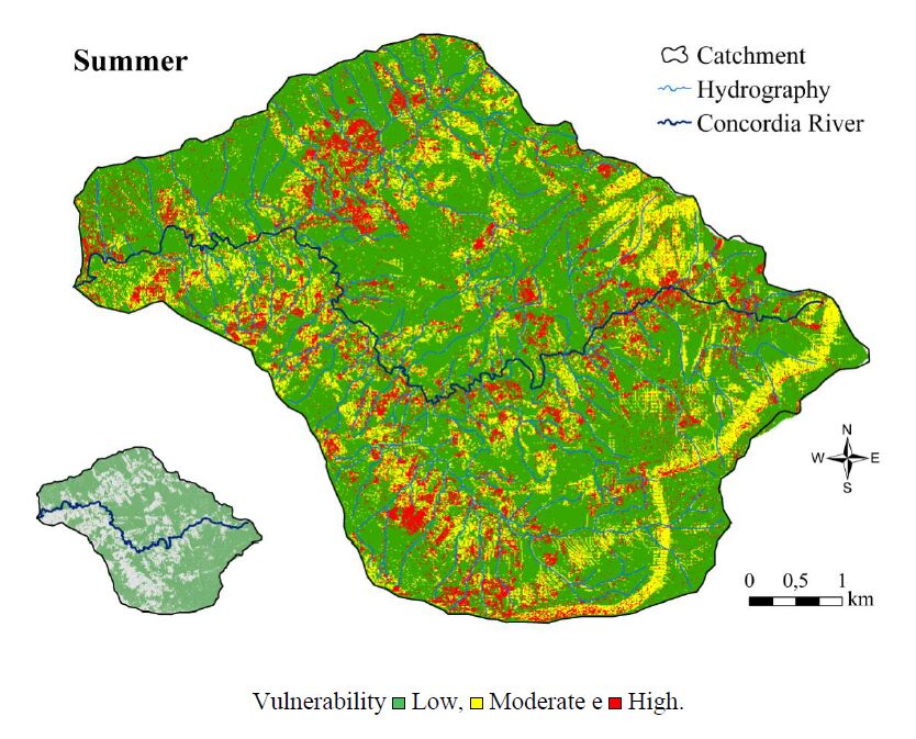
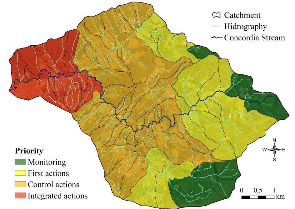
Figures(4) / Tables(10)

Rafael Gotardo, Gustavo A. Piazza, Edson Torres, Vander Kaufmann, Adilson Pinheiro. Soil Loss Vulnerability in an Agricultural Catchment in the Atlantic Forest Biome in Southern Brazil[J]. AIMS Geosciences, 2016, 2(4): 345-365. doi: 10.3934/geosci.2016.4.345

| Cluster Type | |||||||
| Summary statistics (total link strengh) | Orange | Purple | Yellow | Dark Blue | Light Blue | Green | Red |
| Mean | 120.6667 | 137.5 | 120.75 | 134.5 | 149.4286 | 171.1 | 149.5 |
| Std. Dev. | 38.3597 | 79.7102 | 64.8289 | 50.3284 | 56.7094 | 105.9397 | 88.0682 |
| Min. | 62 | 20 | 40 | 64 | 43 | 40 | 20 |
| Max. | 164 | 269 | 233 | 230 | 230 | 448 | 286 |
| Skewness | -0.2611 | 0.0833 | 0.4621 | 0.5460 | -0.6475 | 1.8279 | 0.2911 |
| Kurtosis | 1.9842 | 2.2609 | 2.1889 | 2.4399 | 3.2227 | 6.0794 | 1.7576 |
| IQR | 58 | 102.5 | 92 | 64 | 46 | 30 | 148 |
| Intra-cluster metrics | Orange | Purple | Yellow | Dark Blue | Light Blue | Green | Red |
| Shannon Diversity (H') | 1.7471 | 1.9129 | 1.9523 | 2.2408 | 1.8730 | 2.1558 | 2.6005 |
| Evenness (E) | 0.9751 | 0.9199 | 0.9389 | 0.9732 | 0.9625 | 0.9362 | 0.9379 |
| Richness (S) | 6 | 8 | 8 | 10 | 7 | 10 | 16 |
| Inter-cluster outcomes | Orange | Purple | Yellow | Dark Blue | Light Blue | Green | Red |
| Orange ('materialistic-based') cluster | 1 | ||||||
| Purple ('firm-driven') cluster | 1.9613∗∗∗(9.0981)[1807] | 1 | |||||
| Yellow ('regional marketing-based') cluster | 1.9614∗∗∗(10.9347)[1625] | 1.9611∗(1.8539)[2041] | 1 | ||||
| Dark Blue ('ideology-based') cluster | 1.9613∗∗∗(34.2942)[1734] | 1.9612∗∗∗(18.7034)[1942] | 1.9614∗∗∗(15.9394)[1677] | 1 | |||
| Light Blue ('university-driven') cluster | 1.9614∗∗∗(8.4344)[1683] | 1.9612∗∗(2.2210)[1954] | 1.9613∗∗∗(2837)[1713] | 1.9610∗∗∗(26.1370)[2294] | 1 | ||
| Green ('sustainability-driven') cluster | 1.9610∗∗∗(24.0138)[2317] | 1.9609∗∗∗(12.3030)[2528] | 1.9610∗∗∗(10.0489)[2228] | 1.9608∗∗∗(5.2233)[2947] | 1.9608∗∗∗(16.8875)[2757] | 1 | |
| Red ('consumption-driven') cluster | 1.9610∗∗∗(56.2142)[2208] | 1.9610∗∗∗(37.8203)[2280] | 1.9612∗∗∗(34.6116)[1945] | 1.9606∗∗∗(25.0826)[3627] | 1.9608∗∗∗(48.9103)[2989] | 1.9606∗∗∗(26.2031)[3594] | 1 |
| Notes: *** p<0.01 ** p<0.05 * p<0.1. In relation to inter-cluster diversity outcomes, coefficient estimates are presented without parenthesis or brackets, t-statistics are displayed in parentheses and degrees of freedom are observed in brackets. IQR denotes interquartile range. | |||||||
DownLoad:
CSV
| Consumption | Country-of-origin/city | Environment | Ideology | Materialism | University | |
| I. Statistical tests | ||||||
| Frequency | 1/5 | 5/12 | 7/60 | 11/60 | 1/20 | 1/30 |
| Suest-based Hausman | ϰ2[12]=4.494p=0.973 | ϰ2[12]=3.645p=0.989 | ϰ2[12]=4.980p=0.959 | ϰ2[12]=2.499p=0.998 | ϰ2[12]=1.705p=1.000 | ϰ2[12]=2.290p=0.999 |
| Individual significanceΨ | ϰ2[5]=14.830∗∗p=0.011 | ϰ2[5]=4.360p=0.499 | ϰ2[5]=12.160∗∗p=0.033 | ϰ2[5]=7.240p=0.203 | ϰ2[5]=5.850p=0.321 | ϰ2[5]=3.810p=0.577 |
| II. Coefficients | ||||||
| Consumption cluster normalized to zero | ||||||
| Intercept | 1.116∗∗(0.491) | −1.230(0.837) | 1.167(0.532) | 0.251(0.647) | −1.643(1.115) | |
| Topic 1 | −1.805∗∗(0.872) | −1.229(1.651) | −4.421∗∗∗(1.625) | −3.559∗(2.036) | −1.698(2.690) | |
| Topic 2 | 1.130(2.545) | 6.474∗∗(2.853) | −2.618∗∗(3.545) | −3.117(5.821) | 5.536∗(3.141) | |
| III. Marginal effects at the mean | ||||||
| Topic 1 | 0.508∗∗(0.203) | 0.017(0.270) | 0.080(0.179) | −0.506∗∗(0.223) | −0.106(0.122) | 0.007(0.111) |
| Topic 2 | −0.220(0.516) | 0.210(0.535) | 0.721∗∗(0.324) | −0.672∗(0.403) | −0.245(0.207) | 0.206(0.197) |
| IV. Qualitative metrics | ||||||
| Log Likelihood | −69.217 | |||||
| Notes: *** p<0.01 ** p<0.05 * p<0.1. Non-robust standard errors in parentheses since the method of estimation is maximum likelihood. The symbol Ψ serves to indicate that the joint significance test result for all regressors is ϰ2[30]=39.110 with p=0.123, the joint significance test result for all regressors except for Topics 1 and 2 is ϰ2[20]=19.180 with p=0.510 and the joint significance test result only for Topics 1 and 2 is ϰ2[10]=21.390 with p=0.019, thereby justifying the final deterministic component of the regression model β1+β2Topic1i+β3Topic2i for a critical p-value of 5%, with i={Article 1,...,Article 60}. | ||||||
DownLoad:
CSV
| Author | Article | Area of research | Year | Topic |
| Karrh (1998) | Brand placement: A review | Business, Management and Accounting | 1998 | Review of place branding and related variants |
| Dinnie et al. (2004a) | Place branding: Overview of an emerging literature | Business, Management and Accounting | 2004 | Review of place branding and related variants |
| Dinnie et al. (2004b) | Country-of-origin 1965-2004: A literature review | Business, Management and Accounting | 2004 | Review of the country-of-origin theme |
| Guzman (2005) | A brand building literature review | Social Sciences | 2005 | Generical review on brand building |
| Chabowski et al. (2013) | A bibliometric analysis of the global branding literature and a research agenda | Social Sciences | 2013 | Bibliometric analysis of global branding |
| Papadopoulos et al. (2016) | Nation branding for foreign direct investment:an Integrative review and directions for research and strategy | Business and Economics | 2016 | Review of nation brand literaturefocusing on FDI |
| White et al. (2016) | Trends in international strategic management research from 2000 to 2013:Text mining and bibliometric analyses | Business, Management and Accounting | 2016 | Review of strategic management researchwith a brief coverage of nation image |
| Hao et al. (2021) | Two decades of research on nation branding: A review and future research agenda | Business, Management and Accounting | 2021 | Review of country branding |
| He et al. (2021) | Building the connection between nation and commercial brand:an integrative review and future research directions | Business, Management and Accounting | 2021 | Proposal of a coordination frameworkbetween nation and commercial branding |
| Södergren (2021) | Brand authenticity: 25 Years of research | Business, Management and Accounting | 2021 | Review on brand autheticity |
| Rojas-Méndez and Khoshnevis (2023) | Conceptualizing nation branding: the systematic literature review | Business, Management and Accounting | 2023 | Systematic literature review on nation branding |
DownLoad:
CSV
| [Ranking] Authors (Year) | Title | Journal | Cited by |
| [1] Mooij (2003) | Convergence and divergence in consumer behaviour: Implications for global advertising | International Journal of Advertising | 88 |
| [2] Matzler et al. (2016) | Brand personality and culture: The role of cultural differences on the impact of brand personality perceptions on tourists' visit intentions | Tourism Management | 87 |
| [3] Anholt (2005) | Anholt nation brands index: How does the world see America? | Journal of Advertising Research | 58 |
| [4] Gupta (2011) | Globalization does lead to change in consumer behavior: An empirical evidence of impact of globalization on changing materialistic values in Indian consumers and its aftereffects | Asia Pacific Journal of Marketing and Logistics | 49 |
| [5] Foscht et al. (2008) | The impact of culture on brand perceptions: A six-nation study | Journal of Product&Brand Management | 49 |
| [6] Rojas-Méndez (2016) | The nation brand molecule | Journal of Product&Brand Management | 29 |
| [7] Geary (2013) | Incredible India in a global age: The cultural politics of image branding in tourism | Tourist Studies | 25 |
| [8] Hsieh and Lindridge (2005) | Universal appeals with local specifications | Journal of Product&Brand Management | 22 |
| [9] Clifton (2014) | Towards a holistic understanding of county of origin effects? Branding of the region, branding from the region | Journal of Destination Marketing and Management | 18 |
| [10] Wilson and Hollensen (2010) | Saipa Group, Iran - using strategic brand extensions to build relationships | Journal of Islamic Marketing | 18 |
| [11] Gong et al. (2014) | Global use and access of social networking web sites: A national culture perspective | Journal of Research in Interactive Marketing | 15 |
| [12] Bulmer and Buchanan-Oliver (2010) | Experiences of brands and national identity | Australasian Marketing Journal | 14 |
| [13] Therkelsen and Gram (2010) | Branding Europe - between nations, regions and continents | Scandinavian Journal of Hospitality and Tourism | 12 |
| [14] Pearson and Pearson (2017) | Branding Food Culture: UNESCO Creative Cities of Gastronomy | Journal of Food Products Marketing | 11 |
| [15] Perez et al. (2011) | Intergenerational influence on brand preferences | Journal of Product & Brand Management | 11 |
| [16] Kaufmann and Durst (2008) | Developing inter-regional brands | EuroMed Journal of Business | 11 |
| [17] Martínez (2016) | Towards a network place branding through multiple stakeholders and based on cultural identities: The case of "The Coffee Cultural Landscape" in Colombia | Journal of Place Management and Development | 10 |
| [18] Song and Sung (2013) | Antecedents of nation brand personality | Corporate Reputation Review | 10 |
| [19] Smith and West (1994) | The globalization of furniture industries/markets | Journal of Global Marketing | 10 |
DownLoad:
CSV
| Description | Results |
| Timespan | 1992 : 2021 |
| Sources (Journals, Books, etc) | 45 |
| Documents | 60 |
| Annual Growth Rate % | 2.42 |
| Document Average Age | 10.5 |
| Average citations per doc | 10.67 |
| Average citations per year per doc | 0.8208 |
| References | 2989 |
| Keywords Plus (ID) | 23 |
| Author's Keywords (DE) | 221 |
| Authors | 133 |
| Author Appearances | 142 |
| Authors of single-authored docs | 19 |
| Single-authored docs | 19 |
| Documents per Author | 0.451 |
| Co-Authors per Doc | 2.37 |
| International co-authorships % | 21.67 |
DownLoad:
CSV
| Cluster Type | |||||||
| Summary statistics (total link strengh) | Orange | Purple | Yellow | Dark Blue | Light Blue | Green | Red |
| Mean | 120.6667 | 137.5 | 120.75 | 134.5 | 149.4286 | 171.1 | 149.5 |
| Std. Dev. | 38.3597 | 79.7102 | 64.8289 | 50.3284 | 56.7094 | 105.9397 | 88.0682 |
| Min. | 62 | 20 | 40 | 64 | 43 | 40 | 20 |
| Max. | 164 | 269 | 233 | 230 | 230 | 448 | 286 |
| Skewness | -0.2611 | 0.0833 | 0.4621 | 0.5460 | -0.6475 | 1.8279 | 0.2911 |
| Kurtosis | 1.9842 | 2.2609 | 2.1889 | 2.4399 | 3.2227 | 6.0794 | 1.7576 |
| IQR | 58 | 102.5 | 92 | 64 | 46 | 30 | 148 |
| Intra-cluster metrics | Orange | Purple | Yellow | Dark Blue | Light Blue | Green | Red |
| Shannon Diversity (H') | 1.7471 | 1.9129 | 1.9523 | 2.2408 | 1.8730 | 2.1558 | 2.6005 |
| Evenness (E) | 0.9751 | 0.9199 | 0.9389 | 0.9732 | 0.9625 | 0.9362 | 0.9379 |
| Richness (S) | 6 | 8 | 8 | 10 | 7 | 10 | 16 |
| Inter-cluster outcomes | Orange | Purple | Yellow | Dark Blue | Light Blue | Green | Red |
| Orange ('materialistic-based') cluster | 1 | ||||||
| Purple ('firm-driven') cluster | 1.9613∗∗∗(9.0981)[1807] | 1 | |||||
| Yellow ('regional marketing-based') cluster | 1.9614∗∗∗(10.9347)[1625] | 1.9611∗(1.8539)[2041] | 1 | ||||
| Dark Blue ('ideology-based') cluster | 1.9613∗∗∗(34.2942)[1734] | 1.9612∗∗∗(18.7034)[1942] | 1.9614∗∗∗(15.9394)[1677] | 1 | |||
| Light Blue ('university-driven') cluster | 1.9614∗∗∗(8.4344)[1683] | 1.9612∗∗(2.2210)[1954] | 1.9613∗∗∗(2837)[1713] | 1.9610∗∗∗(26.1370)[2294] | 1 | ||
| Green ('sustainability-driven') cluster | 1.9610∗∗∗(24.0138)[2317] | 1.9609∗∗∗(12.3030)[2528] | 1.9610∗∗∗(10.0489)[2228] | 1.9608∗∗∗(5.2233)[2947] | 1.9608∗∗∗(16.8875)[2757] | 1 | |
| Red ('consumption-driven') cluster | 1.9610∗∗∗(56.2142)[2208] | 1.9610∗∗∗(37.8203)[2280] | 1.9612∗∗∗(34.6116)[1945] | 1.9606∗∗∗(25.0826)[3627] | 1.9608∗∗∗(48.9103)[2989] | 1.9606∗∗∗(26.2031)[3594] | 1 |
| Notes: *** p<0.01 ** p<0.05 * p<0.1. In relation to inter-cluster diversity outcomes, coefficient estimates are presented without parenthesis or brackets, t-statistics are displayed in parentheses and degrees of freedom are observed in brackets. IQR denotes interquartile range. | |||||||
| Consumption | Country-of-origin/city | Environment | Ideology | Materialism | University | |
| I. Statistical tests | ||||||
| Frequency | 1/5 | 5/12 | 7/60 | 11/60 | 1/20 | 1/30 |
| Suest-based Hausman | ϰ2[12]=4.494p=0.973 | ϰ2[12]=3.645p=0.989 | ϰ2[12]=4.980p=0.959 | ϰ2[12]=2.499p=0.998 | ϰ2[12]=1.705p=1.000 | ϰ2[12]=2.290p=0.999 |
| Individual significanceΨ | ϰ2[5]=14.830∗∗p=0.011 | ϰ2[5]=4.360p=0.499 | ϰ2[5]=12.160∗∗p=0.033 | ϰ2[5]=7.240p=0.203 | ϰ2[5]=5.850p=0.321 | ϰ2[5]=3.810p=0.577 |
| II. Coefficients | ||||||
| Consumption cluster normalized to zero | ||||||
| Intercept | 1.116∗∗(0.491) | −1.230(0.837) | 1.167(0.532) | 0.251(0.647) | −1.643(1.115) | |
| Topic 1 | −1.805∗∗(0.872) | −1.229(1.651) | −4.421∗∗∗(1.625) | −3.559∗(2.036) | −1.698(2.690) | |
| Topic 2 | 1.130(2.545) | 6.474∗∗(2.853) | −2.618∗∗(3.545) | −3.117(5.821) | 5.536∗(3.141) | |
| III. Marginal effects at the mean | ||||||
| Topic 1 | 0.508∗∗(0.203) | 0.017(0.270) | 0.080(0.179) | −0.506∗∗(0.223) | −0.106(0.122) | 0.007(0.111) |
| Topic 2 | −0.220(0.516) | 0.210(0.535) | 0.721∗∗(0.324) | −0.672∗(0.403) | −0.245(0.207) | 0.206(0.197) |
| IV. Qualitative metrics | ||||||
| Log Likelihood | −69.217 | |||||
| Notes: *** p<0.01 ** p<0.05 * p<0.1. Non-robust standard errors in parentheses since the method of estimation is maximum likelihood. The symbol Ψ serves to indicate that the joint significance test result for all regressors is ϰ2[30]=39.110 with p=0.123, the joint significance test result for all regressors except for Topics 1 and 2 is ϰ2[20]=19.180 with p=0.510 and the joint significance test result only for Topics 1 and 2 is ϰ2[10]=21.390 with p=0.019, thereby justifying the final deterministic component of the regression model β1+β2Topic1i+β3Topic2i for a critical p-value of 5%, with i={Article 1,...,Article 60}. | ||||||
| Author | Article | Area of research | Year | Topic |
| Karrh (1998) | Brand placement: A review | Business, Management and Accounting | 1998 | Review of place branding and related variants |
| Dinnie et al. (2004a) | Place branding: Overview of an emerging literature | Business, Management and Accounting | 2004 | Review of place branding and related variants |
| Dinnie et al. (2004b) | Country-of-origin 1965-2004: A literature review | Business, Management and Accounting | 2004 | Review of the country-of-origin theme |
| Guzman (2005) | A brand building literature review | Social Sciences | 2005 | Generical review on brand building |
| Chabowski et al. (2013) | A bibliometric analysis of the global branding literature and a research agenda | Social Sciences | 2013 | Bibliometric analysis of global branding |
| Papadopoulos et al. (2016) | Nation branding for foreign direct investment:an Integrative review and directions for research and strategy | Business and Economics | 2016 | Review of nation brand literaturefocusing on FDI |
| White et al. (2016) | Trends in international strategic management research from 2000 to 2013:Text mining and bibliometric analyses | Business, Management and Accounting | 2016 | Review of strategic management researchwith a brief coverage of nation image |
| Hao et al. (2021) | Two decades of research on nation branding: A review and future research agenda | Business, Management and Accounting | 2021 | Review of country branding |
| He et al. (2021) | Building the connection between nation and commercial brand:an integrative review and future research directions | Business, Management and Accounting | 2021 | Proposal of a coordination frameworkbetween nation and commercial branding |
| Södergren (2021) | Brand authenticity: 25 Years of research | Business, Management and Accounting | 2021 | Review on brand autheticity |
| Rojas-Méndez and Khoshnevis (2023) | Conceptualizing nation branding: the systematic literature review | Business, Management and Accounting | 2023 | Systematic literature review on nation branding |
| [Ranking] Authors (Year) | Title | Journal | Cited by |
| [1] Mooij (2003) | Convergence and divergence in consumer behaviour: Implications for global advertising | International Journal of Advertising | 88 |
| [2] Matzler et al. (2016) | Brand personality and culture: The role of cultural differences on the impact of brand personality perceptions on tourists' visit intentions | Tourism Management | 87 |
| [3] Anholt (2005) | Anholt nation brands index: How does the world see America? | Journal of Advertising Research | 58 |
| [4] Gupta (2011) | Globalization does lead to change in consumer behavior: An empirical evidence of impact of globalization on changing materialistic values in Indian consumers and its aftereffects | Asia Pacific Journal of Marketing and Logistics | 49 |
| [5] Foscht et al. (2008) | The impact of culture on brand perceptions: A six-nation study | Journal of Product&Brand Management | 49 |
| [6] Rojas-Méndez (2016) | The nation brand molecule | Journal of Product&Brand Management | 29 |
| [7] Geary (2013) | Incredible India in a global age: The cultural politics of image branding in tourism | Tourist Studies | 25 |
| [8] Hsieh and Lindridge (2005) | Universal appeals with local specifications | Journal of Product&Brand Management | 22 |
| [9] Clifton (2014) | Towards a holistic understanding of county of origin effects? Branding of the region, branding from the region | Journal of Destination Marketing and Management | 18 |
| [10] Wilson and Hollensen (2010) | Saipa Group, Iran - using strategic brand extensions to build relationships | Journal of Islamic Marketing | 18 |
| [11] Gong et al. (2014) | Global use and access of social networking web sites: A national culture perspective | Journal of Research in Interactive Marketing | 15 |
| [12] Bulmer and Buchanan-Oliver (2010) | Experiences of brands and national identity | Australasian Marketing Journal | 14 |
| [13] Therkelsen and Gram (2010) | Branding Europe - between nations, regions and continents | Scandinavian Journal of Hospitality and Tourism | 12 |
| [14] Pearson and Pearson (2017) | Branding Food Culture: UNESCO Creative Cities of Gastronomy | Journal of Food Products Marketing | 11 |
| [15] Perez et al. (2011) | Intergenerational influence on brand preferences | Journal of Product & Brand Management | 11 |
| [16] Kaufmann and Durst (2008) | Developing inter-regional brands | EuroMed Journal of Business | 11 |
| [17] Martínez (2016) | Towards a network place branding through multiple stakeholders and based on cultural identities: The case of "The Coffee Cultural Landscape" in Colombia | Journal of Place Management and Development | 10 |
| [18] Song and Sung (2013) | Antecedents of nation brand personality | Corporate Reputation Review | 10 |
| [19] Smith and West (1994) | The globalization of furniture industries/markets | Journal of Global Marketing | 10 |
| Description | Results |
| Timespan | 1992 : 2021 |
| Sources (Journals, Books, etc) | 45 |
| Documents | 60 |
| Annual Growth Rate % | 2.42 |
| Document Average Age | 10.5 |
| Average citations per doc | 10.67 |
| Average citations per year per doc | 0.8208 |
| References | 2989 |
| Keywords Plus (ID) | 23 |
| Author's Keywords (DE) | 221 |
| Authors | 133 |
| Author Appearances | 142 |
| Authors of single-authored docs | 19 |
| Single-authored docs | 19 |
| Documents per Author | 0.451 |
| Co-Authors per Doc | 2.37 |
| International co-authorships % | 21.67 |
